
I’ve been looking for a system that can provide fast & accurate position measurement within a defined area; this is generally known as an RTLS (Real Time Location System).
My previous experiments have involved optical measurements, which have good accuracy, but are constrained by line-of-sight and range issues. So why not use wireless, and measure the time it takes for a radio pulse to travel from transmitter to receiver? Given the speed of light is roughly 300 mm (or 1 foot) per nanosecond, it may seem impossible to get an accurate position that way, but Decawave claim that their DW1000 time-of-flight chip gives measurements around 100 mm (4 inch) accuracy, using an Ultra Wideband (UWB) radio.
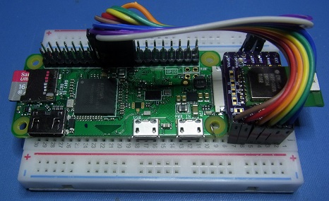
The DWM1000 module is bottom-left in the photo above, and consists of the DW1000 chip with a crystal reference, voltage regulator and on-board antenna. The other two boards use the same wireless chip, in different form-factors, but with additional embedded CPUs. I wanted to experiment with the DW1000 chip in a wide range of scenarios, and fully understand its low-level operation, so decided to use the simpler DWM1000 module, driven by my own Python code.
Decawave provide a large amount of documentation on their chip, and several software packages, but these are quite large: for example, their DecaRanging application has over 20,000 lines of C and C++ source code, which is a bit intimidating if you’re a newcomer to sub-nanosecond radio timing.
So I’ve created a Python test framework from scratch; at under 1000 lines of code, it can’t compete with the Decawave packages, but hopefully it’ll give an insight as to how the chip works, and enable you to experiment with this interesting technology.
Ultra Wideband
You may not have seen this RF technology before, but it has been around a while; the IEEE standard 802.15.4a is dated 2007. Just because it is part of the 802.15.4 family, you may think it is similar to Zigbee or 6LoWPAN, but that is not true. The RF operation is completely different: instead of transmitting on a single frequency, it covers a wide spectrum. This makes it much more resistant to single-frequency interferers, but of course raises the prospect that the UWB transmitter could interfere with other radio systems nearby.
For this reason, there are some quite complex rules about which frequencies can be used, the permissible power-levels, and the transmit repetition-rate. So it is possible that the RF emissions generated by my software are not permitted in your locality. If in doubt, consult a suitably-qualified RF engineer before doing any UWB testing.
Tags and Anchors

The standard Location System consists of several ‘anchors’, which are positioned at known locations, and ‘tags’ which move around a defined area; they determine their position by measuring the transit-time of the signals from several anchors.
This scheme works well for, say, locating people within a shopping mall; their mobile phones can be the tags, displaying the location within that mall – and non-coincidentally, the Apple iPhone 11 does have an UWB capability.
An alternative scenario is where the tags are fitted to vehicles in a warehouse, allowing a management system to track their whereabouts. There are two ways this can be achieved; either a tag just transmits a simple beacon message, and the anchors share their time-measurements to establish its position, or alternatively the tag measures its distance from the nearest anchors, and transmits the result for forwarding to the management system.
Implicitly, a tag is a battery powered device that only transmits occasionally, but in reality there are many other ways to configure a location network, depending on the overall requirements.
This flexibility comes from the fact that the ranging messages can also carry data (up to 127 bytes as standard), so there are numerous ways the RTLS can be structured. In this first post, I’m ignoring all that complexity, and just focusing on the distance measurement between two systems, which could be tags, anchors, or anything else you decide.
Ranging
Ranging is the process whereby two UWB radio systems can measure the distance between themselves. Simplistically, one might think that it is just necessary for the transmitter to note the time of a message transmission, and the receiver to note the time it is received: subtract the two and you get a time-difference, which is directly proportional to the distance between them.
However, it isn’t quite that simple, because:
- The measurement has to be very accurate; a radio wave travels at around 300,000,000 metres per second (1 foot per nanosecond) so to achieve any degree of accuracy, we need a time measurement in picoseconds (10-12 seconds).
- In this method, the time-clocks of the transmitter and receiver have to be very accurately synchronised, and that isn’t easy.
- To keep hardware costs down, each of the units will have an inexpensive quartz crystal as the timing reference, and we have to accommodate variations in the crystal frequency due to its tolerance, temperature drift, etc.
- The radio wave that arrives at the receiver won’t be an accurate copy of what is transmitted; there will be distortions due to the radio circuitry, and reflections from nearby objects.
Fortunately, these problems can be addressed by using a technique called ‘Asymmetric Two Way Ranging’:
- Use very fast, high-resolution timers; the sampling clock on the the DW1000 runs at 63.8976 GHz, and feeds a 40-bit counter.
- Don’t synchronise the clocks in the transmitter and receiver; let them just free-run.
- Measure the difference in crystal frequency, and compensate for it.
- Use Ultra-Wideband (UWB) which is more resilient than conventional radio systems.

In the diagram above, there are 3 messages passing between two units; unit A transmits messages 1 and 3, unit B sends message 2. Each unit records a timestamp when the message was sent or received, so we have a total of 6 timestamps, from which to determine the transit time, and hence the distance.
Simplistically the transit time can be measured by comparing Rx2 – Tx1 with Tx2 – Rx1, but you’ll see that the time clocks for units A and B are running at different speeds. In reality they’ll only differ by a few parts per million (the difference has been greatly magnified for the illustration) but a small difference creates in a large position error, so we need a method to compensate for it. This is done by getting the two units to make the same measurement, and comparing the result; the obvious candidate is the time between the two transmissions (Tx3 – Tx1) and the time between the two receptions (Rx3 – Rx1). These should be equal, so the ratio of the times will be the ratio of their clock frequencies.
The final formula for the transit time (taken from Decwave’s APS013 application note) is:
rnd1 = Rx2 - Tx1 # Round-trip 1 to 2
rep1 = Tx2 - Rx1 # Reply time 1 to 2
rnd2 = Rx3 - Tx2 # Round-trip 2 to 3
rep2 = Tx3 - Rx2 # Reply time 2 to 3
time = (rnd1 × rnd2 - rep1 * rep2) / (rnd1 + rnd2 + rep1 + rep2)
Hardware

The Decawave DW1000 chip can be purchased from electronic distributors, but unless you’re into microwave PCB design, you’ll want to buy a pre-packaged module. The simplest of these is the DWM1000, which includes the necessary power circuitry and ceramic chip antenna. It has no on-board CPU, so is driven by an external processor over a 4-wire Serial Peripheral Interface (SPI).
You could solder wires direct to the package, but I used an adaptor board that brings out the connections to a breadboard-friendly 0.1″ pitch. The adaptor is the “DWM1000 Breakout-01”, available from OSH Park.
Aside from the SPI interface (CLK, MISO, MOSI and CS) you only have to provide 3.3V power and ground, though I also connected reset (RST) and interrupt (IRQ) signals. Reset is very useful to clear down the chip before programming, and the interrupt saves the chip from frenetic polling during transmission or reception (which can disrupt the RF section of some chips).
Which CPU to drive the module? Any microcontroller would do, but I’d like to control the modules using a single Python program on a PC; this is much easier than updating multiple copies of the software on different CPUs. So I’m attaching each module to a Raspberry Pi, to act as a relatively dumb network-to-SPI converter; I can then send streams of SPI commands from the PC program over a WiFi network to 2 or more UWB modules, without having to reprogram their CPUs.
SPI port 0 or 1 can be used on the RPi, so long as it is enabled in /boot/config/txt. The pin numbers are:
# Connector pin numbers:
#       SPI0        SPI1
# GND   25          34
# CS    24 (CE0)    36 (CE2)
# MOSI  19          38
# MISO  21          35
# CLK   23          40
# IRQ   18          32
# RESET 22 (BCM25)  37 (BCM26)
# NRST  16 (BCM23)  31 (BCM6)
# 3.3V  17
I have provided a positive-going reset signal (RESET) and negative-going (NRST). This is because my early hardware had a transistor inverter in the reset line, so needed a positive-going signal. If you are connecting the RPi pin direct to the module, use the NRST signal. [And in case you’re wondering, I realise that the RPi mustn’t drive the module reset line high; my software does not do this, it drives the line low to reset, or lets it float.]
A useful extra is to fit an LED indicator to the module interrupt line (with a current-limiting resistor of a few hundred ohms to ground). This will flash in a recognisable pattern when ranging is working correctly, which is very useful when testing the module’s operational limits.
The module with a Pi ZeroW and USB power pack is a neat package; I had some concerns about taking 3.3V power from the RPi, due to possible electrical noise issues, but it seems to work fine, providing you keep the cable to the module short – I’d suggest a maximum of 100 mm (4 inches) if you want to avoid problems.
Raspberry Pi Software

We need a simple way of sending commands to the network nodes from the PC; since each command is a small data block, and we have to wait for the command to be executed before sending the next, the logical choice is User Datagram Protocol (UDP). This is an ‘unreliable’ protocol, as it has no mechanism for retrying any lost transmissions, or eliminating any duplicates, so I’ve added a lightweight client-server error-handling layer. Each data block (‘datagram’ in UDP parlance) has a 1-byte sequence number, a 1-byte length, and a payload of up to 255 bytes. The client (PC system) increments the sequence number with each new transmission; the server (Raspberry Pi) checks whether that sequence number has already been received. If so, the data is ignored, and the previous response is just resent; if not, the data is sent to the UWB module over the SPI interface, and the response is returned to the client.
Network Server
The code on the Raspberry Pi has been kept simple; it is single-threaded by using the ‘select’ mechanism to poll the socket for incoming data, with a timeout that allows the interrupt indicator to be polled:
import socket, select

# Simple UDP server
class Server(object):
    def __init__(self):
        self.rxdata, self.txdata = [], []
        self.sock = self.addr = None

    # Open socket
    def open(self, portnum):
        self.sock = socket.socket(socket.AF_INET, socket.SOCK_DGRAM)
        self.sock.setsockopt(socket.SOL_SOCKET, socket.SO_REUSEADDR, 1)
        self.sock.bind(('', portnum))
        return self.sock

    # Receive incoming data with timeout
    def recv(self, maxlen=MAXDATA, timeout=SOCK_TIMEOUT):
        rxdata = []
        socks = [self.sock]
        rd, wr, ex = select.select(socks, [], [], timeout)
        for s in rd:
            rxdata, self.addr = s.recvfrom(maxlen)
        return rxdata

    # Receive incoming request, return iterator for data blocks
    # If sequence number is unchanged, resend last transmission
    def receive(self):
        self.rxdata = bytearray(self.recv(MAXDATA))
        if len(self.rxdata) > SEQLEN:
            if len(self.txdata)>SEQLEN and self.rxdata[0]==self.txdata[0]:
                self.xmit(self.txdata)
            else:
                self.txdata = [self.rxdata[0]]
                rxd = self.rxdata[SEQLEN-1:]
                while len(rxd)>1 and len(rxd)>rxd[0]:
                    n = rxd[0] + 1
                    yield(rxd[1:n])
                    rxd = rxd[n:]

    # Add response data to list
    def send(self, data):
        self.txdata += [len(data)] + data

    # Transmit responses
    def xmit(self, txdata, suffix=''):
        if self.addr and len(txdata)>SEQLEN:
            txd = bytearray(txdata)
            self.sock.sendto(txd, self.addr)
SPI interface
This consists of a clock line, data from the RPi to the module (MOSI: Master Out Slave In), data from the module (MISO: Master In Slave Out) and a Chip Select (CS) line that frames each transmission.
For protocol details, see the Decawave DW1000 datasheet. The most significant bit of the first byte indicates a read or write cycle; a read cycle returns one or more garbage bytes (depending on the addressing mode) followed by the actual data; my software returns all of these bytes back to the PC. A write-cycle returns no useful data (it is generally all-ones) but this is still passed back to the PC, as an acknowledgement that the write command has been received.
import spidev, RPi.GPIO as GPIO

# Open SPI interface
spif = 0,0
spi = spidev.SpiDev()
spi.open(*spif)
spi.max_speed_hz = 2000000
spi.mode = 0

# Set up board I/O
rst_pin, irq_pin = 22, 18
GPIO.setmode(GPIO.BOARD)
GPIO.setwarnings(False)
GPIO.setup(rst_pin, GPIO.OUT)
GPIO.setup(irq_pin, GPIO.IN)
GPIO.add_event_detect(irq_pin, GPIO.RISING, callback=irq_handler)
The clock speed of 2 MHz is well within the specified limits for the module. The interrupt (IRQ) line is high when asserted, so positive-edge-detection is used; the callback just sets a global variable that is polled in the main loop.
Running code on startup
It is convenient for the SPI server code to automatically run when the RPi boots; there are various ways to do this, which are beyond the scope of this blog. I used systemd as follows:
sudo systemctl edit --force --full spi_server.service

# Add the following to spi_server.service..
 [Unit]
   Description=SPI server
   Wants=network-online.target
   After=network-online.target
 [Service]
   Type=simple
   User=pi
   WorkingDirectory=/home/pi/uwb
   ExecStart=/usr/bin/python spi_server.py
 [Install]
   WantedBy=multi-user.target

# Enable the service using:
sudo systemctl enable spi_server.service
sudo systemctl start spi_server.service  # ..or 'stop' to stop it

# To check if service is running..
systemctl status spi_server
Main Program
This Python program (dw1000_range.py) runs on a PC, feeding command strings over the network to the Raspberry Pi UDP-to-SPI adaptors.
Device Initialisation
The bulk of the main program is involved in device initialisation, as the DW1000 has a remarkably large number of registers – my software defines 106, and that isn’t all of them. To add to the complexity, they vary in size between 1 and 14 bytes, have multiple bitfields within them, and are accessed by a multi-level addressing scheme.
By any measure, this is a complex chip, and is a very easy for the software to degenerate into endless sequences of ANDing SHIFTing and ORing to insert new data into a register. To avoid this, the C language has bitfields, and the equivalent in Python is ‘ctypes’, indeed this library was created to allow Python to access DLLs written in C.
I’ve used ctypes in a novel way to give a clean way of reading & writing one or more fields of a register, without any cumbersome logic operations.
To give a simple example, DW1000 register 0 is 32 bits wide, containing a 4-bit revision number in the least significant bits, then a 4-bit version, 8-bit model, and a 16-bit tag number.
I have defined this as:
DEV_ID = 0x0, 4, None, (("REV", U32, 4), ("VER",   U32, 4),
                        ("MODEL",U32, 8), ("RIDTAG",U32,16))
This data is passed to a Python class:
from ctypes import LittleEndianStructure as Structure, Union
from ctypes import c_uint as U32, c_ulonglong as U64

# DW1000 register class
class Reg(object):
    def __init__(self, regdef, val=0):
        self.name, self.value = regdef, val
        self.id, self.len, self.sub, self.fields = globals()[regdef]
        class struct(Structure):
            _fields_ = self.fields
        class union(Union):
            _fields_ = [("reg", struct), ("value", U64)]
        self.u = union()
        self.u.value = val
        self.reg = self.u.reg

    # Read register value
    def read(self, spi):
        # [Do SPI read cycle]
        return self

    # Write register value
    def write(self, spi):
        # [Do SPI write cycle]
        return self

# Set a field within a register
    def set(self, field, val):
        if hasattr(self.reg, field):
            setattr(self.reg, field, val)
        else:
            print("Unknown attribute: '%s'" % field)
        self.value = self.u.value
        return self
The union overlays an array of bytes on top of the register value; this provides a byte data-stream to be used by the SPI read & write functions.
Instantiating the class gives us a local copy of the DW1000 register, and the ‘read’ method populates the copy with values from the remote register, e.g.
r = Reg('DEV_ID')
r.read(spi)
print("%X" % r.reg.RIDTAG)
Note that the class methods return ‘self’, so can be chained; for example, here is a read-modify-write cycle that sets the transmit frame length, which is in the bottom 7 bits of the 40-bit register 8:
TX_FCTRL  = 0x8, 5, None,(("TFLEN", U64, 7), ("TFLE", U64, 3), ("R", U64, 3),
                          ("TXBR",  U64, 2), ("TR",   U64, 1), ("TXPRF", U64, 2),
                          ("TXPSR", U64, 2), ("PE",   U64, 2), ("TXBOFFS", U64, 10),
                          ("IFSDELAY",  U64, 8))

Reg('TX_FCTRL').read(spi).set('TFLEN', txlen).write(spi)
‘spi’ in these examples is a class instance that contains the code to read or write the SPI interface; in my test framework, this is actually a network interface that sends the data to a Raspberry Pi, and obtains the response. This is necessary because I have one Python program controlling two (or more) DW1000 modules, so I need a class instance for each SPI interface, giving an IP address and UDP port number, e.g.
# Class for an SPI interface
class Spi(object):
    def __init__(self, spif, ident='1'):
        self.spif, self.ident = spif, ident
        self.txseq = 0
        self.verbose = self.interrupt = False
        self.sock = socket.socket(socket.AF_INET, socket.SOCK_DGRAM)
        if self.sock:
            self.sock.connect(spif[1:])
            print("Connected to %s:%u" % spif[1:])
        else:
            print("Can't open socket")

SPIF = "UDP", "10.1.1.226", 1401
print("Connecting to %s port %s:%u" % SPIF)
spi = Spi(SPIF)
Before leaving the subject of device initialisation, it is worth mentioning that I’ve used several Python dictionaries (as lookup tables) to simplify the underlying logic: for example, the transmitter analog setting RF_TXCTRL, which depends on the channel number (1 – 7, excluding 6)
CHAN_RF_TXCTRL  = {1:0x5c40, 2:0x45ca0, 3:0x86cc0, 4:0x45c80, 5:0x1e3fe0, 7:0x1e7de0}
Reg('RF_TXCTRL', CHAN_RF_TXCTRL[chan]).write(self.spi)
The register class is instantiated using a value from the dictionary, then that value is written to the hardware.
There is a drawback to my approach; the maximum size of any register is limited to 64 bits (c_ulonglong). Fortunately there are only 2 registers longer than this (RX_TIME: 14 bytes, TX_TIME: 10 bytes) and these can be split into sections to come within the 8-byte limit.
Frame Format
A transmitted message (‘frame’) consists of a preamble that the receiver will synchronise to, a start-of-frame delimiter (SFD), and the data payload. The preamble & SFD are automatically inserted by the DW1000, and are used by the timing logic to produce an accurate timestamp, so generally the recommended values will be used. The data payload, however, can be anything; if you want to inter-operate with other UWB 802.15.4 devices it can be a maximum of 127 bytes and must have a standardised header; if not, it can be any format up to 1023 bytes.
Normally, the payload would be used to convey timing information from a tag to an anchor, but in my case the main Python program has visibility of all data through the Wifi network, so I don’t need to send any data across UWB. Arbitrarily, I chose to send the data of an 802.15.4 ‘blink’, which is a very short message containing a 1-byte prefix, 1-byte sequence number and 8-byte address.
# Blink frame with IEEE EUI-64 tag ID
BLINK_FRAME_CTRL = 0xc5
BLINK_MSG=(('framectrl',   U8),
           ('seqnum',      U8),
           ('tagid',       U64))
This is instantiated using a Frame class that is similar to the Reg class described above, allowing us to refer to the fields individually, or collectively as a stream of bytes.
blink1 = Frame(BLINK_MSG)
blink1.values.framectrl = BLINK_FRAME_CTRL
blink1.values.tagid = 0x0101010101010101
txdata = blink1.data()
Transmission
Having done all the hard work initialising the chip, transmission is just a question of setting the frame data & length, then setting a single bit.
dw1 = DW1000(spi1)
dw1.initialise()
dw1.set_txdata(txdata)
dw1.start_tx()
The timing-specific information is handled automatically, so the precise time of the transmission (specifically, the timing of the SFD) can be determined by a single function call:
    # Get Tx timestamp
    def tx_time(self):
        return Reg('TX_TIME1').read(self.spi).reg.TX_STAMP
You can set the hardware to generate an interrupt (IRQ signal) when transmission is complete, but I haven’t found this necessary.
Reception
To receive a frame, the preamble, SFD and data must be decoded; the data must pass a CRC check, and the address must match the filtering criteria if these are enabled. Success or failure is signalled by various bits in the SYS_STATUS register; these bits can also be used to signal an interrupt, if enabled in the SYS_MASK register. In my code, the following signals are enabled as interrupts:
- RXPHE: phy header error
- RXFCG: receiver frame check good
- RXFCE: receiver frame check eror
- RXRFSL: receiver frame sync loss
- RXRFTO: receiver frame wait timeout
- RXSFDTO: receive SFD timeout
- AFFREJ: automatic frame filtering reject
The most important signals are RXFCG / RXFCE to signal a good frame, or an error condition. The Decawave code has complex error handling, to tackle some ways in which the chip might lock up, and stop responding. Since we have one master program controlling both transmission and reception, we can adopt a simplistic approach to error handling, and if a chip fails to receive several consecutive transmissions, it is reset and re-initialised.
Assuming reception is successful, the data and timestamp can be read out; in our case, we’re only really interested in the time:
    # In DW1000 class..
    def get_rxdata(self):
        rxdata = []
        if self.check_interrupt():
            status = Reg('SYS_STATUS').read(self.spi)
            if status.reg.RXDFR:
                rxdata = self.rx_data()
        return rxdata

    # Get Rx timestamp
    def rx_time(self):
        return Reg('RX_TIME1').read(self.spi).reg.RX_STAMP
...
rxdata = dw1.get_rxdata()
dt1 = dw1.rx_time() - dw1.tx_time()
dt2 = dw2.tx_time() - dw2.rx_time()
Running the test
The Python source files are on Github, they are:
Main PC program:
- dw1000_range.py: main program to run the test
- dw1000_regs.py: classes describing the UWB chip internals
- dw1000_spi.py: SPI-over-UDP interface
Raspberry Pi:
- spi_server.py
The files are compatible with Python 2.7 or 3.x
I didn’t get around to providing a neat UI on the main program, so at the top of dw1000_range.py you have to enter the IP addresses of the two RPi units, e.g.
# Specify SPI interfaces:
#   "UDP", "<IP_ADDR>", <PORT_NUM>
SPIF1       = "UDP", "10.1.1.235", 1401
SPIF2       = "UDP", "10.1.1.230", 1401
There is an optional verbose ‘-v’ command-line flag that enables the display of all the incoming & outgoing data. This includes a modulo-10-second timestamp with 1 millisecond resolution, which is useful for tracking down timing problems.
The SPI server running on the RPi units has a similar ‘-v’ option for verbose mode, and an optional port number that also changes the SPI interface, so port 1401 can be SPI0, and 1402 can be SPI1.
To run the test, first make sure the SPI servers are running on the 2 RPis; you can run them from ssh consoles, but I have found that this noticeably degrades the UDP response times on a Pi Zero (see the ‘potential problems’ section below) so once you’ve proved they work, I’d recommend running the code on startup, as described above.
Then run the main program; you should see a stream of ranging results, e.g.
Connected to 10.1.1.226:1401
Connected to 10.1.1.230:1401
147.136 156.569
146.991 156.616
147.127 156.602
146.053 156.555
144.017 156.555
146.001 156.588
..and so on..
This is from 2 units 2 metres (6.5 feet) apart. The first column is the distance in metres for simple 2-message ranging with no measurement of the difference in clock frequencies; the second column is for full asymmetric ranging, that uses a total of 3 messages to compensate for clock inaccuracies.
I’ve said that the units are 2 metres apart, so you’d expect a value of 2 to be displayed, not 147 or 156. The reason for this discrepancy is that the RF circuitry adds a very large time-delay to the signal, that has to be subtracted from the final result. The best way to calculate this compensation value is to measure several known distances, and adjust the multiplier and constant values to produce the right answers.
I haven’t done this calibration process yet, so the un-adjusted result is displayed. The main focus of my current test is to see how repeatable the results are, i.e. how much jitter there is in the position value.
Taking 1000 readings, at distances between 2 and 6 metres, (roughly 6.5 to 20 feet) produces the following histogram of the error between the actual distance (as indicated by the average of all the samples) and the reported distance:

You’ll see the error doesn’t get much greater as the distance increases, i.e. it is not a percentage of the distance measured. This shows that (under good-signal conditions) the main error source is the jitter in the capture and measurement of the incoming wave, as discussed in the Decawave literature, and this is relatively constant irrespective of distance.
The above tests are in good line-of-sight conditions, so to degrade the signal I did a 9 metre (30 foot) range test obstructed by a sizeable brick wall (1900-vintage, not a flimsy modern partition) and a few items of furniture. To my surprise, the error histogram didn’t show very much degradation.

It is also worth noting that despite the convoluted control and measurement process (PC talking to Raspberry Pis), around 5 ranging results are returned per second. Using local CPUs (as in many of the Decawave demonstration systems) will produce a major speed improvement, and a simple rolling average would markedly improve the position accuracy.
Potential problems
Here are some issues you may encounter:
- Power supply. In my experience, the most common problem is with the power supply. When receiving or transmitting, the Decawave module takes around 160 milliamps, which is more than some simple 3.3V supplies can handle. Also, the module may appear to work, even if the power supply is completely disconnected; the startup current is sufficiently low that the module can power itself from the I/O lines, and return a valid ID across the SPI interface, even though it is unpowered. Of course it will fail as soon as any real operations start, but the initial SPI response may lead you to look for complex bugs in your code, rather than a simple power supply fault.
- IRQ. The software does include a check that the interrupt (IRQ) line is operational, by setting it as an output, then toggling it; see the ‘pulse_irq’ method. If this check fails, there is no point proceeding with the tests.
- Missed interrupts. After each transmission, the main software waits for 50 milliseconds to get an interrupt from the receiving unit; if this doesn’t arrive, it polls the receiver’s status register, and if an interrupt is pending (i.e. the message has been received), it reports ‘missed interrupt’. This is harmless, and could be disabled; the reason is that the Raspberry Pi networking stack occasionally adds a long delay to UDP transmissions. To see this in action, try sending flood pings from the RPi to a fast server; I’ve seen round-trip times vary between 3 and 80 msec, even if the WiFi network is very lightly loaded, and the RPi is doing nothing else.
- Hardware Reset. Whilst not essential for the testing, if the reset line isn’t connected, things can get confusing, since the chip won’t be cleared down between tests, and the software does assume a ‘clean slate’ at the start of the test.
- Status display. If reception fails with error flags set, I display the receiver status; this information is useful in formulating an error-handling strategy.
- Bursts of failures. Sometimes when seeing a poor signal, the units stop communicating, and rack up continuous errors. If my software detects 10 such errors, it resets the two units, then carries on as normal. This is not the correct approach; if you look at the Decawave source code, they check the status register to look for potential lock-up conditions, and take appropriate action; they don’t wait for multiple failures.
- RF performance. Another weakness of my approach is that it doesn’t represent an accurate simulation of the RF performance of the Decawave chips. Radio circuitry needs decent RF design, and putting a module with an adaptor PCB on a breadboard is not good from an RF perspective. It is credit to the Decwave designers that their module tolerates this approach, producing reasonable results – but if they fall short of expectations, don’t be too surprised; to get the best from the chips and modules, proper hardware design is required.
Ultra-Wideband is a remarkable technology, and I’ve only scratched the surface of what it can do; now see what you can make of it…
Copyright (c) Jeremy P Bentham 2019. Please credit this blog if you use the information or software in it.
