Web display for Pi Pico oscilloscope

Web oscilloscope display

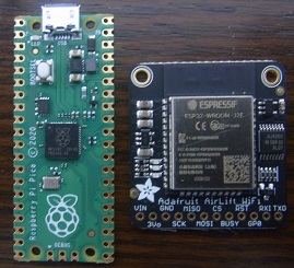
In part 1 of this series, I added WiFi connectivity to the Pi Pico using an ESP32 moduleand MicroPython. Part 2 showed how Direct Memory Access (DMA) can be used to get analog samples at regular intervals from the Pico on-board Analog Digital Converter (ADC).

I’m now combining these two techniques with some HTML and Javascript code to create a Web display in a browser, but since this code will be quite complicated, first I’ll sort out how the data is fetched from the Pico Web server.

Data request

The oscilloscope display will require user controls to alter the sample rate, number of samples, and any other settings we’d like to change. These values must be sent to the Web server, along with a filename that will trigger the acquisition. To fetch 1000 samples at 10000 samples per second, the request received by the server might look like:

GET /capture.csv?nsamples=1000&xrate=10000

If you avoid any fancy characters, the Python code in the server that extracts the filename and parameters isn’t at all complicated:

ADC_SAMPLES, ADC_RATE = 20, 100000
parameters = {"nsamples":ADC_SAMPLES, "xrate":ADC_RATE}

# Get HTTP request, extract filename and parameters
req = esp.get_http_request()
if req:
    line = req.split("\r")[0]
    fname = get_fname_params(line, parameters)

# Get filename & parameters from HTML request
def get_fname_params(line, params):
    fname = ""
    parts = line.split()
    if len(parts) > 1:
        p = parts[1].partition('?')
        fname = p[0]
        query = p[2].split('&')
        for param in query:
            p = param.split('=')
            if len(p) > 1:
                if p[0] in params:
                    try:
                        params[p[0]] = int(p[1])
                    except:
                        pass
    return fname

The default parameter names & values are stored in a dictionary, and when the URL is decoded, and names that match those in the dictionary will have their values updated. Then the data is fetched using the parameter values, and returned in the form of a comma-delimited (CSV) file:

if CAPTURE_CSV in fname:
    vals = adc_capture()
    esp.put_http_text(vals, "text/csv", esp32.DISABLE_CACHE)

The name ‘comma-delimited’ is a bit of a misnomer in this case, we just with the given number of lines, with one floating-point voltage value per line.

Requesting the data

Before diving into the complexities of graphical display and Javascript, it is worth creating a simple Web page to fetch this data.

The standard way of specifying parameters with a file request is to define a ‘form’ that will be submitted to the server. The parameter values can be constrained using ‘select’, to avoid the user entering incompatible numbers:

<html><!DOCTYPE html><html lang="en">
<head><meta charset="utf-8"/></head><body>
  <form action="/capture.csv">
    <label for="nsamples">Number of samples</label>
    <select name="nsamples" id="nsamples">
      <option value=100>100</option>
      <option value=200>200</option>
	  <option value=500>500</option>
      <option value=1000>1000</option>
    </select>
    <label for="xrate">Sample rate</label>
    <select name="xrate" id="xrate">
      <option value=1000>1000</option>
      <option value=2000>2000</option>
	  <option value=5000>5000</option>
      <option value=10000>10000</option>
    </select>
	<input type="submit" value="Submit">
  </form>
</body></html>

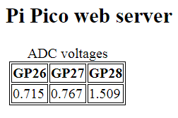
This generates a very simple display on the browser:

Form to request ADC samples

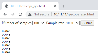
On submitting the form, we get back a raw list of values:

CSV data

Since the file we have requested is pure CSV data, that is all we get; the controls have vanished, and we’ll have to press the browser ‘back’ button if we want to retry the transaction. This is quite unsatisfactory, and to improve it there are various techniques, for example using a template system to always add the controls at the top of the data. However, we also want the browser to display the data graphically, which means a sizeable amount of Javascript, so we might as well switch to a full-blown AJAX implementation, as mentioned in the first part.

AJAX

To recap, AJAX originally stood for ‘Asynchronous JavaScript and XML’, where the Javascript on the browser would request an XML file from the server, then display data within that file on the browser screen. However, there is no necessity that the file must be XML; for simple unstructured data, CSV is adequate.

The HTML page is similar to the previous one, the main changes are that we have specified a button that’ll call a Javascript function when clicked, and there is a defined area to display the response data; this is tagged as ‘preformatted’ so the text will be displayed in a plain monospaced style.

  <form id="captureForm">
    <label for="nsamples">Number of samples</label>
    <select name="nsamples" id="nsamples">
      <option value=100>100</option>
      <option value=200>200</option>
	  <option value=500>500</option>
      <option value=1000>1000</option>
    </select>
    <label for="xrate">Sample rate</label>
    <select name="xrate" id="xrate">
      <option value=1000>1000</option>
      <option value=2000>2000</option>
	  <option value=5000>5000</option>
      <option value=10000>10000</option>
    </select>
    <button onclick="doSubmit(event)">Submit</button>
  </form>
  <pre><p id="responseText"></p></pre>

The button calls the Javascript function ‘doSubmit’ when clicked, with the click event as an argument. As this button is in a form, by default the browser would attempt to re-fetch the current document using the form data, so we need to block this behaviour and substitute the action we want, which is to wait until the response is obtained, and display it in the area we have allocated. This is ‘asynchronous’ (using a callback function) so that the browser doesn’t stall waiting for the response.

function doSubmit() {
  // Eliminate default action for button click
  // (only necessary if button is in a form)
  event.preventDefault();

  // Create request
  var req = new XMLHttpRequest();

  // Define action when response received
  req.addEventListener( "load", function(event) {
    document.getElementById("responseText").innerHTML = event.target.responseText;
  } );

  // Create FormData from the form
  var formdata = new FormData(document.getElementById("captureForm"));

  // Collect form data and add to request
  var params = [];
  for (var entry of formdata.entries()) {
    params.push(entry[0] + '=' + entry[1]);
  }
  req.open( "GET", "/capture.csv?" + encodeURI(params.join("&")));
  req.send();
}

The resulting request sent by the browser looks something like:

GET /capture.csv?nsamples=100&xrate=1000

This is created by looping through the items in the form, and adding them to the base filename. When doing this, there is a limited range of characters we can use, in order not to wreck the HTTP request syntax. I have used the ‘encodeURI’ function to encode any of these unusable characters; this isn’t necessary with simple parameters that are just alphanumeric values, but if I’d included a parameter with free-form text, this would be needed. For example, if one parameter was a page title that might include spaces, then the title “Test page” would be encoded as

GET /capture.csv?nsamples=100&xrate=1000&title=Test%20page

You may wonder why I am looping though the form entries, when in theory they can just be attached to the HTTP request in one step:

// Insert form data into request - doesn't work!
req.open("GET", "/capture.csv");
req.send(formdata);

I haven’t been able to get this method to work; I think the problem is due to the way the browser adapts the request if a form is included, but in the end it isn’t difficult to iterate over the form entries and add them directly to the request.

The resulting browser display is a minor improvement over the previous version, in that it isn’t necessary to use the ‘back’ button to re-fetch the data, but still isn’t very pretty.

Partial display of CSV data

Graphical display

There many ways to display graphic content within a browser. The first decision is whether to use vector graphics, or a bitmap; I prefer the former, since it allows the display to be resized without the lines becoming jagged.

There is a vector graphics language for browsers, namely Scalable Vector Graphics (SVG) and I have experimented with this, but find it easier to use Javascript commands to directly draw on a specific area of the screen, known as an ‘HTML canvas’, that is defined within the HTML page:

<div><canvas id="canvas1"></canvas></div>

To draw on this, we create a ‘2D context’ in Javascript:

var ctx1 = document.getElementById("canvas1").getContext("2d");

We can now use commands such as ‘moveto’ and ‘lineto’ to draw on this context; a useful first exercise is to draw a grid across the display.

var ctx1, xdivisions=10, ydivisions=10, winxpad=10, winypad=30;
var grid_bg="#d8e8d8", grid_fg="#40f040";
window.addEventListener("load", function() {
  ctx1 = document.getElementById("canvas1").getContext("2d");
  resize();
  window.addEventListener('resize', resize, false);
} );

// Draw grid
function drawGrid(ctx) {
  var w=ctx.canvas.clientWidth, h=ctx.canvas.clientHeight;
  var dw = w/xdivisions, dh=h/ydivisions;
  ctx.fillStyle = grid_bg;
  ctx.fillRect(0, 0, w, h);
  ctx.lineWidth = 1;
  ctx.strokeStyle = grid_fg;
  ctx.strokeRect(0, 1, w-1, h-1);
  ctx.beginPath();
  for (var n=0; n<xdivisions; n++) {
    var x = n*dw;
    ctx.moveTo(x, 0);
    ctx.lineTo(x, h);
  }
  for (var n=0; n<ydivisions; n++) {
    var y = n*dh;
    ctx.moveTo(0, y);
    ctx.lineTo(w, y);
  }
  ctx.stroke();
}

// Respond to window being resized
function resize() {
  ctx1.canvas.width = window.innerWidth - winxpad*2;
  ctx1.canvas.height = window.innerHeight - winypad*2;
  drawGrid(ctx1);
}

I’ve included a function that resizes the canvas to fit within the window, which is particularly convenient when getting a screen-grab for inclusion in a blog post:

All that remains is to issue a request, wait for the response callback, and plot the CSV data onto the canvas.

var running=false, capfile="/capture.csv"

// Do a single capture (display is done by callback)
function capture() {
  var req = new XMLHttpRequest();
  req.addEventListener( "load", display);
  var params = formParams()
  req.open( "GET", capfile + "?" + encodeURI(params.join("&")));
  req.send();
}

// Display data (from callback event)
function display(event) {
  drawGrid(ctx1);
  plotData(ctx1, event.target.responseText);
  if (running) {
    window.requestAnimationFrame(capture);
  }
}

// Get form parameters
function formParams() {
  var formdata = new FormData(document.getElementById("captureForm"));
  var params = [];
  for (var entry of formdata.entries()) {
    params.push(entry[0]+ '=' + entry[1]);
  }
  return params;
}

A handy feature is to have the display auto-update when the current data has been displayed; I’ve done this by using requestAnimationFrame to trigger another capture cycle, if the global ‘running’ variable is set. Then we just need some buttons to control this feature:

<button id="single" onclick="doSingle()">Single</button>
<button id="run"  onclick="doRun()">Run</button>
// Handle 'single' button press
function doSingle() {
  event.preventDefault();
  running = false;
  capture();
}

// Handle 'run' button press
function doRun() {
  event.preventDefault();
  running = !running;
  capture();
}

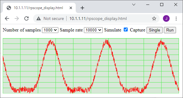
The end result won’t win any prizes for style or speed, but it does serve as a useful basis for acquiring & displaying data in a Web browser.

100 Hz sine wave

You’ll see that the controls have been rearranged slightly, and I’ve also added a ‘simulate’ checkbox; this invokes MicroPython code in the Pico Web server that doesn’t use the ADC; instead it uses the CORDIC algorithm to incrementally generate sine & cosine values, which are multiplied, with some random noise added:

# Simulate ADC samples: sine wave plus noise
def adc_sim():
    nsamp = parameters["nsamples"]
    buff = array.array('f', (0 for _ in range(nsamp)))
    f, s, c = nsamp/20.0, 1.0, 0.0
    for n in range(0, nsamp):
        s += c / f
        c -= s / f
        val = ((s + 1) * (c + 1)) + random.randint(0, 100) / 300.0
        buff[n] = val
    return "\r\n".join([("%1.3f" % val) for val in buff])
Distorted sine wave with random noise added

Running the code

If you haven’t done so before, I suggest you run the code given in the first and second parts, to check the hardware is OK.

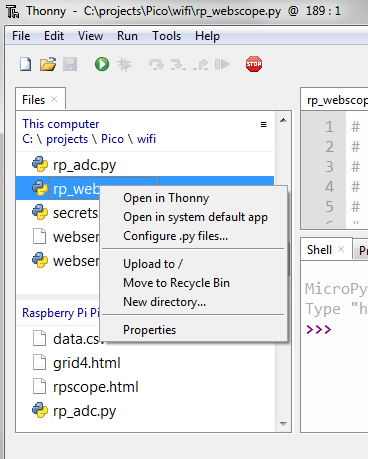
Load rp_devices.py and rp_esp32.py onto the Micropython filesystem, not forgetting to modify the network name (SSID) and password at the top of that file. Then load the HTML files rpscope_capture, rpscope_ajax and rpscope_display, and run the MicroPython server rp_adc_server.py using Thonny. The files are on Github here.

You should then be able to display the pages as shown above, using the IP address that is displayed on the Thonny console; I’ve used 10.1.1.11 in the examples above.

When experimenting with alternative Web pages, I found it useful to run a Web server on my PC, as this allows a much faster development process. There are many ways to do this, the simplest is probably to use the server that is included as standard in Python 3:

python -m http.server 8000

This makes the server available on port 8000. If the Web browser is running on the same PC as the server, use the ‘localhost’ address in the browser, e.g.

http://127.0.0.1:8000/rpscope_display.html

This assumes the HTML file is in the same directory that you used to invoke the Web server. If you also include a CSV file named ‘capture.csv’, then it will be displayed as if the data came from the Pico server.

However, there is one major problem with this approach: the CSV file will be cached by the browser, so if you change the file, the display won’t change. This isn’t a problem on the Pico Web server, as it adds do-not-cache headers in the HTTP response. The standard Python Web server doesn’t do that, so will use the cached data, even after the file has changed.

One other issue is worthy of mention; in my setup, the ESP32 network interface sometimes locks up after it has transferred a significant amount of data, which means the Web server becomes unresponsive. This isn’t an issue with the MicroPython code, since the ESP32 doesn’t respond to pings when it is in this state. I’m using ESP32 Nina firmware v 1.7.3; hopefully, by the time you read this, there is an update that fixes the problem.

Copyright (c) Jeremy P Bentham 2021. Please credit this blog if you use the information or software in it.

Pi Pico wireless Web server using ESP32 and MicroPython

There are various ways that the Pi Pico (RP2040) can be given a wireless interface; in a previous post I used a Microchip ATWINC1500, now I’m using the Espressif ESP32 WROOM-32. The left-hand photo above shows an Adafruit Airlift ESP32 co-processor board which must be hand-wired to the Pico, whilst the right-hand is a Pimorini Wireless Pack that plugs directly into the Pico, either back-to-back, or (as in the photo) on an Omnibus baseboard that allows multiple I/O boards to be attached to a single Pico.

So you can add WiFi connectivity to your Pico without any additional wiring.

The resulting hardware would normally be programmed in C, but I really like the simplicity of MicroPython, so have chosen that language, but this raises an additional question; do I use the Pimorini MicroPython that is derived from the Pi Foundation version, or CircuitPython, which is a derivative created by Adafruit, with various changes?

CircuitPython includes a lot of I/O libraries as standard, but does lack some important features (such as direct access to memory) that are useful to the more advanced developer. So I’ll try to support both, but I do prefer the working with MicroPython.

SPI interface

The ESP32 does all the hard work of connection to the WiFi network and handling TCP/IP sockets, it is just necessary to send the appropriate commands over the SPI link. In addition to the usual clock, data and chip-select lines, there is a ‘reset’ signal from the Pico to the ESP, and a ‘ready’ signal back from the ESP to the Pico. This is necessary because the Pico spends much of its time waiting for the ESP to complete a command; instead of continually polling for a result, the Pico can wait until ‘ready’ is signalled then fetch the data.

My server code uses the I/O pins defined by the Adafruit Pico Wireless Pack:

Function            GPIO  Pin num
Clock               18    24
Pico Tx data (MOSI) 19    25
Pico Rx data (MISO) 16    21
Chip select (CS)     7    10
ESP32 ready         10    14
ESP32 reset         11    15

Software components

Pico software modules and ESP32 interface

ESP32 code

The ESP32 code takes low-level commands over the SPI interface, such as connecting and disconnecting from the wireless network, opening TCP sockets, sending and receiving data. The same ESP32 firmware works with both the MicroPython and CircuitPython code and I suggest you buy an ESP32 module with the firmware pre-loaded, as the re-building & re-flashing process is a bit complicated, see here for the code, and here for a guide to the upgrade process. I’m using 1.7.3, you can check the version in CircuitPython using:

import board
from digitalio import DigitalInOut
esp32_cs = DigitalInOut(board.GP7)
esp32_ready = DigitalInOut(board.GP10)
esp32_reset = DigitalInOut(board.GP11)
spi = busio.SPI(board.GP18, board.GP19, board.GP16)
esp = adafruit_esp32spi.ESP_SPIcontrol(spi, esp32_cs, esp32_ready, esp32_reset)
print("Firmware version", esp.firmware_version.decode('ascii'))

Note that some ESP32 modules are preloaded with firmware that provides a serial interface instead of SPI, using modem-style ‘AT’ commands; this is incompatible with my code, so the firmware will need to be re-flashed.

MicroPython or CircuitPython

This has to be loaded onto the Pico before anything else. There are detailed descriptions of the loading process on the Web, but basically you hold down the Pico pushbutton while making the USB connection. The Pico will then appear as a disk drive in your filesystem, and you just copy (drag-and-drop) the appropriate UF2 file onto that drive. The Pico will then automatically reboot, and run the file you have loaded.

The standard Pi Foundation MicroPython lacks the necessary libraries to interface with the ESP32, so we have to use the Pimorini version. At the time of writing, the latest ‘MicroPython with Pimoroni Libs’ version is 0.26, available on Github here. This includes all the necessary driver code for the ESP32.

If you are using CircuitPython, the installation is a bit more complicated; the base UF2 file (currently 7.0.0) is available here, but you will also need to create a directory in the MicroPython filesystem called adafruit_esp32spi, and load adafruit_esp32spi.py and adafruit_esp32spi_socket.py into it. The files are obtained from here, and the loading process is as described below.

Loading files through REPL

A common source of confusion is the way that files are loaded onto the Pico. I have already described the loading of MicroPython or CircuitPython UF2 images, but it is important to note that this method only applies to the base Python code; if you want to add files that are accessible to your software (e.g. CircuitPython add-on modules, or Web pages for the server) they must be loaded by a completely different method.

When Python runs, it gives you an interactive console, known as REPL (Read Evaluate Print Loop). This is normally available as a serial interface over USB, but can also be configured to use a hardware serial port. You can directly execute commands using this interface, but more usefully you can use a REPL-aware editor to prepare your files and upload them to the Pico. I use Thonny; Click Run and Select Interpreter, and choose either MicroPython (Raspberry Pi Pico) or CircuitPython (Generic) and Thonny will search your serial port to try and connect to Python running on the Pico. You can then select View | Files, and you get a window that shows your local (PC) filesystem, and also the remote Python files. You can then transfer files to & from the PC, and create subdirectories.

At the time of writing, Thonny can’t handle drag-and-drop between the local & remote directories; you have to right-click on a file, then select ‘upload’ to copy it to the currently-displayed remote directory. Do not attempt a transfer while the remote MicroPython program is running; hit the ‘stop’ button first.

In the case of CircuitPython, you need to create a subdirectory called adafruit_esp32spi, containing adafruit_esp32spi.py and adafruit_esp32socket.py.

Server code

To accommodate the differences between the two MicroPython versions, I have created an ESP32 class, with functions for connecting to the wireless network, and handling TCP sockets; it is just a thin wrapper around the MicroPython functions which send SPI commands to the ESP32, and read the responses.

Connecting to the WiFi network just requires a network name (SSID) and password; all the complication is handled by the ESP32. Then a socket is opened to receive the HTTP requests; this is normally on port 80.

def start_server(self, port):
    self.server_sock = picowireless.get_socket()
    picowireless.server_start(port, self.server_sock, 0)

There are significant differences between conventional TCP sockets, and those provided by the ESP32; there is no ‘bind’ command, and the client socket is obtained by a strangely-named ‘avail_server’ call, which also returns the data length for a client socket – a bit confusing. This is a simplified version of the code:

def get_client_sock(self, server_sock):
    return picowireless.avail_server(server_sock)

def recv_length(self, sock):
    return picowireless.avail_server(sock)

def recv_data(self, sock):
    return picowireless.get_data_buf(sock)

def get_http_request(self):
    self.client_sock = self.get_client_sock(self.server_sock)
    client_dlen = self.recv_length(self.client_sock)
    if self.client_sock != 255 and client_dlen > 0:
        req = b""
        while len(req) < client_dlen:
            req += self.recv_data(self.client_sock)
        request = req.decode("utf-8")
        return request
    return None

When the code runs, the IP address is printed on the console

Connecting to testnet...
WiFi status: connecting
WiFi status: connected
Server socket 0, 10.1.1.11:80

Entering the IP address (10.1.1.11 in the above example) into a Web browser means that the server receives something like the following request:

GET / HTTP/1.1
Host: 10.1.1.11
Connection: keep-alive
Cache-Control: max-age=0
Upgrade-Insecure-Requests: 1
User-Agent: Mozilla/5.0 (Windows NT 6.1; Win64; x64) AppleWebKit/537.36 (KHTML, like Gecko) Chrome/93.0.4577.82 Safari/537.36
Accept: text/html,application/xhtml+xml,application/xml;q=0.9,image/avif,image/webp,image/apng,*/*;q=0.8,application/signed-exchange;v=b3;q=0.9
Accept-Encoding: gzip, deflate
Accept-Language: en-GB,en-US;q=0.9,en;q=0.8

Most of this information is irrelevant to a tiny Web server, since there is little choice over the information it returns. The first line has the important information, namely the resource that is being requested, so instead of decoding the whole message, we can do simple tests to match the line to known resources:

DIRECTORY = "/"
INDEX_FNAME   = "rpscope.html"
DATA_FNAME    = "data.csv"
ICON_FNAME    = "favicon.ico"

DISABLE_CACHE = "Cache-Control: no-cache, no-store, must-revalidate\r\n"
DISABLE_CACHE += "Pragma: no-cache\r\nExpires: 0\r\n"

req = esp.get_http_request()
if req:
    r = req.split("\r")[0]
    if ICON_FNAME in r:
        esp.put_http_404()
    elif DATA_FNAME in r:
        esp.put_http_file(DIRECTORY+DATA_FNAME, "text/csv", DISABLE_CACHE)
    else:
        esp.put_http_file(DIRECTORY+INDEX_FNAME)

Since we are dealing with live data, that may change every time it is fetched, the browser’s caching mechanism must be disabled, hence the DISABLE_CACHE response, which aims to do so regardless of which browser version is in use.

Sending the response back to the browser should be easy, it just needs to be split into chunks of maximum 4095 bytes so as to not overflow the SPI buffers. However I had problems with unreliability of both the MicroPython and CircuitPython implementations; sometimes the network transfers would just stall. The solution seems to be to drastically reduce the SPI block size; some CircuitPython code uses 64-byte blocks, but I’ve found 128 bytes works OK. Further work is needed to establish the source of the problem, but this workaround is sufficient for now.

MAX_SPI_DLEN = const(128)
HTTP_OK = "HTTP/1.1 200 OK\r\n"
CONTENT_LEN = "Content-Length: %u\r\n"
CONTENT_TYPE = "Content-type %s\r\n"
HEAD_END = "\r\n"

def put_http_file(self, fname, content="text/html; charset=utf-8", hdr=""):
    try:
        f = open(fname)
    except:
        f = None
    if not f:
        esp.put_http_404()
    else:
        flen = os.stat(fname)[6]
        resp = HTTP_OK + CONTENT_LEN%flen + CONTENT_TYPE%content + hdr + HEAD_END
        self.send_data(self.client_sock, resp)
        n = 0
        while n < flen:
            data = f.read(MAX_SPI_DLEN)
            self.send_data(self.client_sock, data)
            n += len(data)
        self.send_end(self.client_sock)

Dynamic web server

A simple Web server could just receive a page request from a browser, match it with a file in the Pico filesystem, and return the page text to the browser. However, I’d like to report back some live data that has been captured by the Pico, so we need a method to return dynamically-changing values.

There are three main ways of doing this; server-side includes (SSI), AJAX, and on-demand page creation.

Server-side includes

A Web page that is stored in the server filesystem may include tags that trigger the server to perform specific actions, for example when the tag ‘$time’ is reached, the server replaces that text with the current time value. A slightly more sophisticated version embeds the tag in an HTML comment, so the page can be displayed without a Pico server, albeit with no dynamic data.

The great merit of this approach is its simplicity, and I used it extensively in my early projects. However, there is one major snag; the data is embedded in an HTML page, so is difficult to extract. For example, you may have a Web page that contains the temperature data for a 24-hour period, and you want to aggregate that into weekly and monthly reports; you could write a script that strips out the HTML and returns pure data, but it’d be easier if the Web server could just provide a data file for each day.

AJAX

Web pages routinely include Javascript code to perform various display functions, and one of these functions can fetch a data file from the server, and display its contents. This is commonly known as AJAX (Asynchronous Javascript and XML) though in reality there is no necessity for the data to be in XML format; any format will do.

For example, to display a graph of daily temperatures, the Browser loads a Web page with the main formatting, and Javascript code that requests a comma-delimited (CSV) data file. The server prepares that file dynamically using the current data, and returns it to the browser. The Javascript on the browser decodes the data, and displays it as a graph; it can also perform calculations on the data, such as reporting minimum and maximum values.

The key advantage is that the data file can be made available to any other applications, so a logging application can ignore all the Javascript processing, and just fetch the data file directly from the server.

With regard to the data file format, I prefer not to use XML if I can possibly avoid it, so use Javascript Object Notation (JSON) for structured data, and comma-delimited (CSV) for unstructured values, such as data tables.

The first ‘A’ in AJAX stands for Asynchronous, and this deserves some explanation. When the Javascript fetches the data file from the server, there will be a delay, and if the server is heavily loaded, this might be a substantial delay. This could result in the code becoming completely unresponsive, as it waits for data that may never arrive. To avoid this, the data fetching function XMLHttpRequest() returns immediately, but with a callback function that is triggered when the data actually arrives from the server – this is the asynchronous behaviour.

There is now a more modern approach using a ‘fetch’ function that substitutes a ‘promise’ for the callback, but the net effect is the same; keeping the Javascript code running while waiting for data to arrive from the server.

On-demand page creation

The above two techniques rely on the Web page being stored in a filesystem on the server, but it is possible for the server code to create a page from scratch every time it is requested.

Due to the complexity of hand-coding HTML, this approach is normally used with page templates, that are converted on-the-fly into HTML for the browser. However, a template system would add significant complexity to this simple demonstration, so I have used the hand-coding approach to create a basic display of analog input voltages, as shown below.

This data table is created from scratch by the server code, every time the page is loaded:

ADC_PINS = 26, 27, 28
ADC_SCALE = 3.3 / 65536
TEST_PAGE = '''<!DOCTYPE html><html>
    <head><style>table, th, td {border: 1px solid black; margin: 5px;}</style></head>
    <body><h2>Pi Pico web server</h2>%s</body></html>'''

adcs = [machine.ADC(pin) for pin in ADC_PINS]

heads = ["GP%u" % pin for pin in ADC_PINS]
vals = [("%1.3f" % (adc.read_u16() * ADC_SCALE)) for adc in adcs]
th = "<tr><th>" + "</th><th>".join(heads) + "</th></tr>"
tr = "<tr><td>" + "</td><td>".join(vals) + "</td></tr>"
table = "<table><caption>ADC voltages</caption>%s</table>" % (th+tr)
esp.put_http_text(TEST_PAGE % table)

Even in this trivial example, there is significant work in ensuring that the HTML tags are nested correctly, so for pages with any degree of complexity, I’d normally use the AJAX approach as described earlier.

Running the code

The steps are:

  • Connect the wireless module
  • Load the appropriate UF2 file
  • In the case of CircuitPython, load the add-on libraries
  • Get the Web server Python code from Github here. The file rp_esp32.py is for MicroPython with Pimoroni Libraries, and rp_esp32_cp.py is for CircuitPython.
  • Edit the top of the server code to set the network name (SSID) and password for your WiFi network.
  • Run the code using Thonny or any other MicroPython REPL interface; the console should show something like:
Connecting to testnet...
WiFi status: connecting
WiFi status: connected
Server socket 0, 10.1.1.11:80
  • Run a Web browser, and access test.html at the given IP address, e.g. 10.1.1.11/test.html. The console should indicate the socket number, data length, the first line of the HTTP request, and the type of request, e.g.
Client socket 1 len 466: GET /test.html HTTP/1.1 [test page]

The browser should show the voltages of the first 3 ADC channels, e.g.

The Web pages produced by the MicroPython and CircuitPython versions are very similar; the only difference is in the table headers, which either reflect the I/O pin numbers, or the analog channel numbers.

If a file called ‘index.html’ is loaded into the root directory of the MicroPython filesystem, it will be displayed in the browser by default, when no filename is entered in the browser address bar. A minimal index page might look like:

<!doctype html><html><head></head>
  <body>
    <h2>Pi Pico web server</h2>
    <a href="test.html">ADC test</a>
  </body>
</html>

So far, I have only presented very simple Web pages; in the next post I’ll show how to fetch high-speed analog samples using DMA, then combine these with a more sophisticated AJAX functionality to create a Web-based oscilloscope.

Copyright (c) Jeremy P Bentham 2021. Please credit this blog if you use the information or software in it.