Category: ESP32

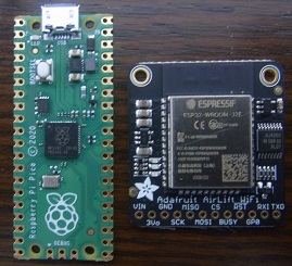
This is the third part of a 3-part blog post describing a low-cost WiFi-based logic analyser, that can be used for monitoring equipment in remote or hazardous locations. Part 1 described the hardware, part 2 the unit firmware, now this post describes the Web interface that controls the logic analyser units, and displays the captured data, also a Python class that can be used to remote-control the units for data analysis.

In a previous post, I experimented with shader hardware (via WebGL) for quickly displaying the logic analyser traces in a Web page. Whilst this technique can provide really fast display updates, there were some browser compatibility problems, and also a pure-javascript version proved to be fast enough, given that the main constraint is the time taken to transfer the data over the network.

So the current solution just used HTML and Javascript, with no hardware acceleration.

Network topology

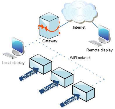
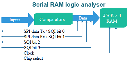
In part 2, I described how the analyser units return data in response to Web page requests; the status information is in the form of a JSON string, and the sample data is Base64 encoded. So each unit has a built-in Web server, and it is tempting to load the HTML display files onto them. However, I chose not to do that, for the following reasons:

• The analyser units use microcontrollers with finite resources, and not much spare storage space.
• Every time the display software is updated, it would have to be loaded onto all the units individually.
• It is easier to keep a single central server up-to-date with all the necessary security & access control measures.

So I’m assuming that there is a Web server somewhere on the system that serves the display file, and any necessary library files. This is a bit inconvenient for development, so when debugging I run a Web server on my development PC, for example using Python 3:

python -m http.server 8000

This launches a server on port 8000; if the display file is in a subdirectory ‘test’, its URL would look like:

http://127.0.0.1:8000/test/remla.html

There is also a question how the display program knows the addresses of the units, so it can access the right one. I had intended to use Multicast DNS (MDNS) for this purpose, but it proved to be a bit unreliable, so I assigned static IP addresses to the units instead.

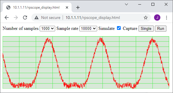
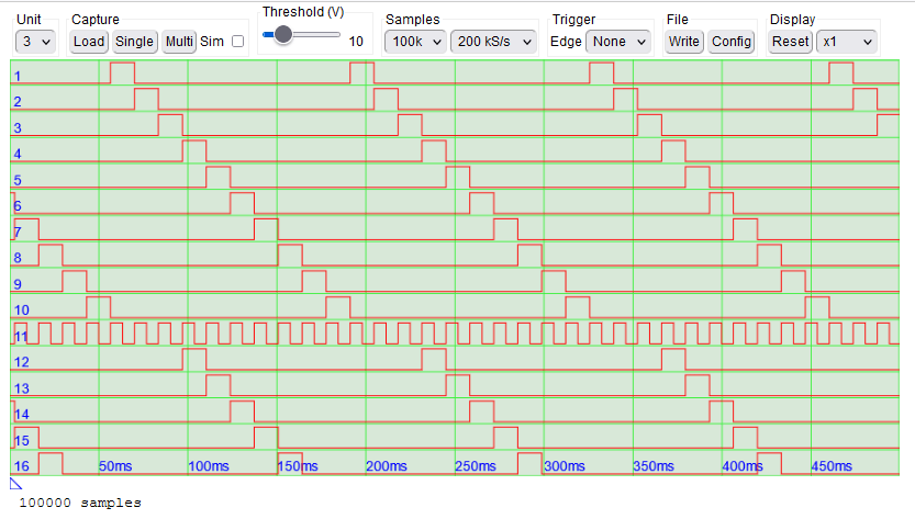
Data display

The waveforms are drawn as vectors (as opposed to bitmaps), so the display can be re-sized to suit any size of screen. There are two basic drawing methods that can be used: an HTML canvas, or SVG (Scalable Vector Graphics). After some experimentation, I adopted the former, as it seemed to be a more flexible solution; the canvas is just an area of the screen that responds to simple line- and text-drawing commands, for example to draw & label the display grid:

var ctx1 = document.getElementById("canvas1").getContext("2d");
drawGrid(ctx1);

// Draw grid in display area
function drawGrid(ctx) {
  var w=ctx.canvas.clientWidth, h=ctx.canvas.clientHeight;
  var dw = w/xdivisions, dh=h/ydivisions;
  ctx.fillStyle = grid_bg;
  ctx.fillRect(0, 0, w, h);
  ctx.lineWidth = 1;
  ctx.strokeStyle = grid_fg;
  ctx.strokeRect(0, 1, w-1, h-1);
  ctx.beginPath();
  for (var n=0; n<xdivisions; n++) {
    var x = n*dw;
    ctx.moveTo(x, 0);
    ctx.lineTo(x, h);
    ctx.fillStyle = 'blue';
    if (n)
        drawXLabel(ctx, x, h-5);
    }
    for (var n=0; n<ydivisions; n++) {
      var y = n*dh;
      ctx.moveTo(0, y);
      ctx.lineTo(w, y);
    }
    ctx.stroke();
  }

Drawing the logic traces uses a similar method; begin a path, add line drawing commands to it, then invoke the stroke method.

Controls

The various control buttons and list boxes need to be part of a form, to simplify the process of sending their values to the analyser unit. So they are implemented as pure HTML:

  <form id="captureForm">
    <fieldset><legend>Unit</legend>
      <select name="unit" id="unit" onchange="unitChange()">
        <option value=1>1</option><option value=2>2</option><option value=3>3</option>
        <option value=4>4</option><option value=5>5</option><option value=6>6</option>
      </select>
    </fieldset>
    <fieldset><legend>Capture</legend>
      <button id="load" onclick="doLoad()">Load</button>
      <button id="single" onclick="doSingle()">Single</button>
      <button id="multi" onclick="doMulti()">Multi</button>
      <label for="simulate">Sim</label>
      <input type="checkbox" id="simulate" name="simulate">
    </fieldset>
..and so on..

To update the parameters on the unit, they are gathered from the form, and sent along with an optional command, e.g. cmd=1 to start a capture.

// Get form parameters
function formParams(cmd) {
  var formdata = new FormData(document.getElementById("captureForm"));
  var params = [];
  for (var entry of formdata.entries()) {
    params.push(entry[0]+ '=' + entry[1]);
  }
  if (cmd != null)
    params.push("cmd=" + cmd);
  return params;
}

// Get status from unit, optionally send command
function get_status(cmd=null) {
  http_request = new XMLHttpRequest();
  http_request.addEventListener("load", status_handler);
  http_request.addEventListener("error", status_fail);
  http_request.addEventListener("timeout", status_fail);
  var params = formParams(cmd), statusfile=remote_ip()+'/'+statusname;
  http_request.open( "GET", statusfile + "?" + encodeURI(params.join("&")));
  http_request.timeout = 2000;
  http_request.send();
}

The result of this HTTP request is handled by callbacks, for example if the request fails, there is a retry mechanism:

// Handle failure to fetch status page
function status_fail(e) {
  var evt = e || event;
  evt.preventDefault();
  if (retry_count < RETRIES) {
    addStatus(retry_count ? "." : " RETRYING")
    get_status();
    retry_count++;
  }
  else {
    doStop();
    redraw(ctx1);
  }
}

This mechanism was found to be necessary since very occasionally the remote unit fails to respond, for no apparent reason; if there is a real reason (e.g. it has been powered down) then the transfer is halted after 3 attempts.

If the status information has been returned OK, then a suitable action is taken; if a capture has been triggered, and the status page indicates that the capture is complete, then the data is fetched:

// Decode status response
function status_handler(e) {
  var evt = e || event;
  var remote_status = JSON.parse(evt.target.responseText);
  var state = remote_status.state;
  if (state != last_state) {
    dispStatus(state_strs[state]);
    last_state = state;
  }
  addStatus(".");
  if (state==STATE_IDLE || state==STATE_PRELOAD || state==STATE_PRETRIG || state==STATE_POSTTRIG) {
    repeat_timer = setTimeout(get_status, 500);
  }
  else if (remote_status.state == STATE_READY) {
    loadData();
  }
  else {
    doStop();
  }
}

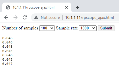
Fetching data

Fetching the data is similar to fetching the status page, since it is a text file containing base64-encoded bytes. The callback converts the text into bytes, then pairs of bytes into an array of numeric values:

// Read captured data (display is done by callback)
function loadData() {
  dispStatus("Reading from " + remote_ip());
  http_request = new XMLHttpRequest();
  http_request.addEventListener("progress", capfile_progress_handler);
  http_request.addEventListener( "load", capfile_load_handler);
  var params = formParams(), capfile=remote_ip()+'/'+capname;
  http_request.open( "GET", capfile + "?" + encodeURI(params.join("&")));
  http_request.send();
}

// Display data (from callback event)
function capfile_load_handler(event) {
  sampledata = getData(event.target.responseText);
  doZoomReset();
  if (command == CMD_MULTI)
    window.requestAnimationFrame(doStart);
  else
    doStop();
}

// Get data from HTTP response
function getData(resp) {
  var d = resp.replaceAll("\n", "");
  return strbin16(atob(d));
}

// Convert string of 16-bit values to binary array
function strbin16(s) {
  var vals = [];
  for (var n=0; n<s.length;) {
    var v = s.charCodeAt(n++);
    vals.push(v | s.charCodeAt(n++) << 8);
  }
  return vals;
}

It is probable that this process could be streamlined somewhat, but currently the main speed restriction is the transfer of data from the ESP to the PC over the wireless network, so improving the byte-decoder wouldn’t give a noticeable speed improvement.

Saving the data

There needs to be some way of saving the sample data for further analysis; as it happens, the initial users of the system were already using the open-source Sigrok Pulseview utility for capturing data from small USB pods, so it was decided to save the data in the Sigrok file format.

This a basically a zipfile, with 3 components:

• Metadata, identifying the channels, sample rate, etc.
• Version, giving the file format version (currently 2)
• Logic file, containing the binary data

The metadata format is quite easy to replicate, e.g.

[global]
sigrok version=0.5.1

[device 1]
capturefile=logic-1
total probes=16
samplerate=5 MHz
total analog=0
probe1=D1
probe2=D2
probe3=D3
..and so on until..
probe16=D16
unitsize=2

The dummy labels D1, D2 etc. are normally replaced with meaningful descriptions of the signals, followed by the unitsize parameter which gives the byte-width of the data, and marks the end of the labels.

The JSZip library is used to zip the various components together in a single file with the ‘sr’ extension:

function write_srdata(fname) {
  var meta = encodeMeta(), zip = new JSZip();
  var samps = new Uint16Array(sampledata);
  zip.file("metadata", meta);
  zip.file("version", "2");
  zip.file("logic-1-1", samps.buffer);
  zip.generateAsync({type:"blob", compression:"DEFLATE"})
  .then(function(content) {
    writeFile(fname, "application/zip", content);
  });
}

// Encode Sigrok metadata
function encodeMeta() {
  var meta=[], rate=elem("xrate").value + " Hz";
  for (var key in sr_dict) {
    var val = key=="samplerate" ? rate : sr_dict[key];
    meta.push(val[0]=='[' ? ((meta.length ? "\n" : "") + val) : key+'='+val);
  }
  for (var n=0; n<nchans; n++) {
    meta.push("probe"+(n+1) + "=" + (probes.length?probes[n]:n+1));
  }
  meta.push("unitsize=2");
  return meta.join("\n");
}

Configuration

So far, the only way the units can be configured is by using the browser controls, to set the sample rate, number of samples, threshold etc. Whilst this might be acceptable for a portable system, a semi-permanent installation needs some way of storing the configuration, including the naming of input channels on the display. Since there is a central Web server for the display files, can’t this also be used to store configuration files? The answer is ‘yes’, but there is then a question how these files can be modified in a browser-friendly way.

This is a bit difficult, since there are numerous security protections for the files on a server, to make sure they can’t be modified by a Web client. However, there is an extension to the HTTP protocol known as WebDAV (Web Distributed Authoring and Versioning), which does provide a mechanism for writing to files. Basically you need a general-purpose Web server that can be configured to support Web DAV (such as lighttpd, see this page), or alternatively a special-purpose server, such as wsgidav (see this page).

Assuming you already have a working lighttpd server, the additional configuration file may look something like this, with some_path, dav_username and dav_password being customised for your installation:

File lighttpd/conf.d/30-webdav.conf:

server.modules += ( "mod_webdav" )
$HTTP["url"] =~ "^/dav($|/)" {
  webdav.activate = "enable"
  webdav.sqlite-db-name = "/some_path/webdav.db"
  server.document-root = "/www/"
  auth.backend = "plain"
  auth.backend.plain.userfile = "/some_path/webdav.shadow"
  auth.require = ("" => ("method" => "basic", "realm" => "webdav", "require" => "valid-user"))
}

File /some_path/webdav.shadow
  dav_username:dav_password
Create directory www/dav for files

Instead, you can use wsgidav to act as a Web and DAV server, run using the Windows command line:

wsgidav.exe --host 0.0.0.0 --port=8000 -c wsgidav.json

The JSON-format configuration file I’m using is:

{
    "host": "0.0.0.0",
    "port": 8080,
    "verbose": 3,
    "provider_mapping": {
        "/": "/projects/remla/test",
        "/test": "/projects/remla/test",
    },
    "http_authenticator": {
        "domain_controller": null,
        "accept_basic": true,
        "accept_digest": true,
        "default_to_digest": true,
        "trusted_auth_header": null
    },
    "simple_dc": {
        "user_mapping": {
            "*": {
                "dav_username": {
                    "password": "dav_password"
                }
            }
        }
    },
    "dir_browser": {
        "enable": true,
        "response_trailer": "",
        "davmount": true,
        "davmount_links": false,
        "ms_sharepoint_support": true,
        "htdocs_path": null
    }
}

Again, this will need to be customised for your environment, and you also need to be mindful that the configurations I’ve shown for lighttpd and wsgidav are quite insecure, for example the password isn’t encrypted, so it can easily be captured by anyone snooping on network traffic.

Configuration Web page

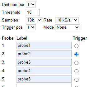
I created a simple Web page to handle the configuration, with list boxes for most options, and text boxes to allow the input channels to be named.

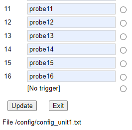
At the bottom of the page there are buttons to submit the new configuration to the server, and exit back to the waveform display page.

The key Javascript function to save the configuration on the server uses the ‘davclient’ library, and is quite simple, but it does need to know the host IP address and port number to receive the data. This code attempts to fetch that information using the DOM Location object:

// Save the config file
function saveConfig() {
  var fname = CONFIG_UNIT.replace('$', String(unitNum()));
  var ip = location.host.split(':')
  var host = ip[0], port = ip[1];
  port = !port ? 80 : parseInt(port);
  var davclient = new davlib.DavClient();
  davclient.initialize(host, port, 'http', DAVUSER, DAVPASS);
  davclient.PUT(fname, JSON.stringify(getFormData()), saveHandler)
 }

For simplicity, the DAV username and password are stored as plain text in the Javascript, which means that anyone viewing the page source can see what they are. This makes the server completely insecure, and must be improved.

Python interface

Although some data analysis can be done in Javascript, it is much more convenient to use Python and its numerical library numpy. I have written a Python class EdlaUnit that provides an API for remote control and data analysis, and a program edla_sweep that demonstrates this functionality.

It repeatedly captures a data block, whilst stepping up the threshold voltage. Then for each block, the number of transitions for each channel is counted and displayed.

import edla_utils as edla, base64, numpy as np

edla.verbose_mode(False)
unit = edla.EdlaUnit(1, "192.168.8")
unit.set_sample_rate(10000)
unit.set_sample_count(10000)

MIN_V, MAX_V, STEP_V = 0, 50, 5

def get_data():
    ok = False
    data = None
    status = unit.fetch_status()
    if status:
        ok = unit.do_capture()
    else:
        print("Can't fetch status from %s" % unit.status_url)
    if ok:
        data = unit.do_load()
    if data == None:
        print("Can't load data")
    return data

for v in range(MIN_V, MAX_V, STEP_V):
    unit.set_threshold(v)
    d = get_data()
    byts = base64.b64decode(d)
    samps = np.frombuffer(byts, dtype=np.uint16)
    diffs = np.diff(samps)
    edges = np.where(diffs != 0)[0]
    totals = np.zeros(16, dtype=int)
    for edge in edges:
        bits = samps[edge] ^ samps[edge+1]
        for n in range(0, 15):
            if bits & (1<<n):
                totals[n] += 1
    s = "%4u," % v
    s += ",".join([("%4u" % val) for val in totals])
    print(s)

The idea is to give a quick overview of the logic levels the analyser is seeing, to make sure they are within reasonable bounds. An example output is:

Volts Ch1  Ch2  Ch3  Ch4  Ch5  Ch6  Ch7  Ch8
0,      0,   0,   0,   0,   0,   0,   0,   0
5,    564, 384, 620, 454, 548, 550, 572, 552
10,   328, 286, 326, 288, 302, 318, 326, 314
15,   260, 246, 262, 244, 260, 254, 260, 250
20,   216, 192, 216, 198, 202, 202, 208, 206
25,    92,   0, 122,   0,  60,  30, 106,  44
30,     0,   0,   0,   0,   0,   0,   0,   0
35,     0,   0,   0,   0,   0,   0,   0,   0
40,     0,   0,   0,   0,   0,   0,   0,   0
45,     0,   0,   0,   0,   0,   0,   0,   0

The absolute count isn’t necessarily very important, since it will vary depending on the signal that is being monitored. What is interesting is the way it changes as the threshold voltage increases. If the number dramatically increases as the ‘1’ logic voltage is approached, one might suspect that there is a noise problem, causing spurious edges. Conversely, if the value declines rapidly before the ‘1’ voltage is reached, the logic level is probably too low.

There is a tendency to assume that all logic signals are a perfect ‘1’ or ‘0’, with nothing in between; this technique allows you to look beyond that, and check whether your signals really are that perfect – and of course you can use the power of Python and numpy to do other analytical tests, or protocol decoding, specific to the signals being monitored.

—

Part 1 of this project looked at the hardware, part 2 the ESP32 firmware. The source files are on Github.

Copyright (c) Jeremy P Bentham 2022. Please credit this blog if you use the information or software in it.

This is the second part of a 3-part blog post describing a low-cost WiFi-based logic analyser, that can be used for monitoring equipment in remote or hazardous locations. Part 1 described the hardware, this post now describes the firmware within the logic analyser unit.

Development environment

There are two main development environments for the ESP32 processor; ESP-IDF and Arduino-compatible. The former is much more comprehensive, but a lot of those features aren’t needed, so to save time, I have used the latter.

There are two ways of developing Arduino code; using the original Arduino IDE, or using Microsoft Visual Studio Code (VS Code) with a build system called PlatformIO. I originally tried to support both, but found the Arduino IDE too restrictive, so opted for VS Code and PlatformIO.

Installing this on Windows is remarkably easy, see these posts on PlatformIO installation or PlatformIO development

Then it is just necessary to open a directory containing the project files, and after a suitable pause while the necessary files are downloaded, the source files can be compiled, and the resulting binary downloaded onto the ESP32 module.

The code has two main areas: driving the custom hardware that captures the samples, and the network interface.

Hardware driver

As described in the previous post, the main hardware elements driven by the CPU are:

• 16-bit data bus for the RAM chips and the comparator outputs
• Clock & chip select for RAM chips
• SPI interface for the DAC that sets the threshold

Data bus

The sample memory consists of four 23LC1024 serial RAM chips, each storing 1 Mbit in quad-SPI (4-bit) mode. They are arranged to form a 16-bit data bus; it would be really convenient if this could be assigned to 16 consecutive I/O bits on the CPU, but the ESP32 hardware does not permit this. The assignment is:

Data line 0  1  2  3  4  5  6  7  8  9 10 11 12 13 14 15
GPIO      4  5 12 13 14 15 16 17 18 19 21 22 23 25 26 27

There is an obvious requirement to handle the data bus as a single 16-bit value within the code, so it is necessary to provide functions that convert that 16-bit data into a 32-bit value to be fed to the I/O pins, and vice-versa, and it’d be helpful if this was done in an easy-to-understand manner, to simplify any changes when a new CPU is used that has a different pin assignment.

After having tried the usual mess of shift-and-mask operations, I hit upon the idea of creating a bitfield for each group of consecutive GPIO pins, and a matching bitfield for the same group in the 16-bit word; then it is only necessary to equate each field to its partner, to produce the required conversion.

// Data bus pin definitions
// z-variables are unused pins
typedef struct {
    uint32_t z1:4, d0_1:2, z2:6, d2_9:8, z3:1, d10_12:3, z4:1, d13_15:3;
} BUSPINS;
typedef union {
    uint32_t val;
    BUSPINS pins;
} BUSPINVAL;

// Matching elements in 16-bit word
typedef struct {
    uint32_t d0_1:2, d2_9:8, d10_12:3, d13_15:3;
} BUSWORD;
typedef union {
    uint16_t val;
    BUSWORD bits;
} BUSWORDVAL;

// Return 32-bit bus I/O value, given 16-bit word
inline uint32_t word_busval(uint16_t val) {
    BUSWORDVAL w = { .val = val };
    BUSPINVAL  p = { .pins = { 0, w.bits.d0_1,   0, w.bits.d2_9,
                               0, w.bits.d10_12, 0, w.bits.d13_15 } };
    return (p.val);
}

// Return 16-bit word, given 32-bit bus I/O value
inline uint16_t bus_wordval(uint32_t val) {
    BUSPINVAL  p = { .val = val };
    BUSWORDVAL w = { .bits = { p.pins.d0_1, p.pins.d2_9, 
                               p.pins.d10_12, p.pins.d13_15 } };
    return (w.val);
}

An additional complication is that the 16-bit value is going to 4 RAM chips, and each chip needs to receive the same command, and the bit-pattern of that command changes depending on whether the chip is in SPI or quad-SPI (QSPI, also known as SQI) mode. So the command to send a command to all 4 RAM chips in SPI mode is:

#define RAM_SPI_DOUT    1
#define MSK_SPI_DOUT    (1 << RAM_SPI_DIN)
#define ALL_RAM_WORD(b) ((b) | (b)<<4 | (b)<<8 | (b)<<12)
uint32_t spi_dout_pins = word_busval(ALL_RAM_WORD(MSK_SPI_DOUT));

// Send byte command to all RAMs using SPI
// Toggles SPI clock at around 7 MHz
void bus_send_spi_cmd(byte *cmd, int len) {
    GPIO.out_w1ts = spi_hold_pins;
    while (len--) {
        byte b = *cmd++;
        for (int n = 0; n < 8; n++) {
            if (b & 0x80) GPIO.out_w1ts = spi_dout_pins;
            else GPIO.out_w1tc = spi_dout_pins;
            SET_SCK;
            b <<= 1;
            CLR_SCK;
        }
    }
}

I have used a ‘bit-bashing’ technique (i.e. manually driving the I/O pins high or low) since I’m emulating 4 SPI transfers in parallel, and as you can see from the comment, the end-result is reasonably fast.

When the RAMS are in QSPI mode, instead of doing eight single-bit transfers, we must do two four-bit transfers:

// Send a single command to all RAMs using QSPI
void bus_send_qspi_cmd(byte *cmd, int len) {
    while (len--) {
        uint32_t b1=*cmd>>4, b2=*cmd&15;
        uint32_t val=word_busval(ALL_RAM_WORD(b1));
        gpio_out_bus(val);
        SET_SCK;
        val = word_busval(ALL_RAM_WORD(b2));
        CLR_SCK;
        gpio_out_bus(val);
        SET_SCK;
        cmd++;
        CLR_SCK;
    }
}

The above code assumes that the appropriate I/O pin-directions (input or output) have been set, but that too depends on which mode the RAMs are in; for SPI each RAM chip has 2 data inputs (DIN and HOLD) and 1 output (DOUT), whilst in QSPI mode all 4 RAM data pins are inputs or outputs depending on whether the RAM is being written to, or read from.

There are 4 commands that the software sends to the RAM chips, each is a single byte:

• 0x38: enter quad-SPI (QSPI) mode
• 0xff: leave QPSI mode, enter SPI mode
• 0x02: write data
• 0x03: read data

The read & write commands are followed by a 3-byte address value, that dictates the starting-point for the transfer. So if the RAMs are already in QSPI mode, the sequence for capturing samples is:

• Set bus pins as outputs, so bus is controlled by CPU
• Assert RAM chip select
• Send command byte, with a value of 2 (write)
• Send 3 address bytes (all zero when starting data capture)
• Set bus pins as inputs, so bus is controlled by comparators
• Start RAM clock
• When capture is complete, stop RAM clock
• Negate RAM chip select

The steps for recovering the captured data are:

• Set bus pins as outputs, so bus is controlled by CPU
• Assert RAM chip select
• Send command byte, with a value of 3 (read)
• Send 3 address bytes
• Set bus pins as inputs, so bus is controlled by the RAM chips
• Toggle clock line, and read data from the 16-bit bus
• When readout is complete, negate RAM chip select

RAM clock and chip select

When the CPU is directly accessing the RAM chips (to send commands, or read back data samples) it is most convenient to ‘bit-bash’ the clock and I/O signals, as described above. It is possible that incoming interrupts can cause temporary pauses in the clock transitions, but this doesn’t matter: the RAM chips use ‘static’ memory, which won’t change its state even if there is a very long pause in a transfer cycle.

However, when capturing data, it is very important that the RAMs receive a steady clock at the required sample rate, with no interruptions. This is easily achieved on the ESP32 by using the LED PWM peripheral:

#define PIN_SCK         33
#define PWM_CHAN        0

// Initialise PWM output
void pwm_init(int pin, int freq) {
    ledcSetup(PWM_CHAN, freq, 1);
    ledcAttachPin(pin, PWM_CHAN);
}

// Start PWM output
void pwm_start(void) {
    ledcWrite(PWM_CHAN, 1);
}
// Stop PWM output
void pwm_stop(void) {
    ledcWrite(PWM_CHAN, 0);
}

In addition, the CPU must count the number of pulses that have been output, so that it knows which memory address is currently being written – there is no way to interrogate the RAM chip to establish its current address value. Surprisingly, the ESP32 doesn’t have a general-purpose 32-bit counter, so we have to use the 16-bit pulse-count peripheral instead, and detect overflows in order to produce a 32-bit value.

volatile uint16_t pcnt_hi_word;

// Handler for PCNT interrupt
void IRAM_ATTR pcnt_handler(void *x) {
    uint32_t intr_status = PCNT.int_st.val;
    if (intr_status) {
        pcnt_hi_word++;
        PCNT.int_clr.val = intr_status;
    }
}

// Initialise PWM pulse counter
void pcnt_init(int pin) {
    pcnt_intr_disable(PCNT_UNIT);
    pcnt_config_t pcfg = { pin, PCNT_PIN_NOT_USED, PCNT_MODE_KEEP, PCNT_MODE_KEEP,
        PCNT_COUNT_INC, PCNT_COUNT_DIS, 0, 0, PCNT_UNIT, PCNT_CHAN };
    pcnt_unit_config(&pcfg);
    pcnt_counter_pause(PCNT_UNIT);
    pcnt_event_enable(PCNT_UNIT, PCNT_EVT_THRES_0);
    pcnt_set_event_value(PCNT_UNIT, PCNT_EVT_THRES_0, 0);
    pcnt_isr_register(pcnt_handler, 0, 0, 0);
    pcnt_intr_enable(PCNT_UNIT);
    pcnt_counter_pause(PCNT_UNIT);
    pcnt_counter_clear(PCNT_UNIT);
    pcnt_counter_resume(PCNT_UNIT);
    pcnt_hi_word = 0;
}

// Return sample counter value (mem addr * 2), extended to 32 bits
uint32_t pcnt_val32(void) {
    uint16_t hi = pcnt_hi_word, lo = PCNT.cnt_unit[PCNT_UNIT].cnt_val;
    if (hi != pcnt_hi_word)
        lo = PCNT.cnt_unit[PCNT_UNIT].cnt_val;
    return(((uint32_t)hi<<16) | lo);
}

When writing this code, I came across some strange features of the PCNT interrupt, such as multiple interrupts for a single event, and misleading values when reading the count value inside the interrupt handler, so be careful when doing any modifications.

The pulse count does not equal the RAM address; is the RAM address multiplied by 2. This is because it takes two 4-bit write cycles to create one byte in RAM (bits 4-7, then 0-3), so the memory chip increments its RAM address once for every 2 samples.

All the RAMs share a single clock line and chip select; the select line is driven low at the start of a command, and must remain low for the duration of the command and data transfer; when it goes high, the transfer is terminated.

Setting threshold value

The comparators compare the incoming signal with a threshold value, to determine if the value is 1 or 0 (above or below threshold). The threshold is derived from a digital-to-analog converter (DAC), the part I’ve chosen is the Microchip MCP4921; it was necessary to use a part with an SPI interface, since there is only 1 spare output pin, which serves as the chip select for this device; the clock and data pins are shared with the RAM chips.

This means that the DAC control code can use the same drivers as the RAM chips by negating the RAM chip select, and asserting the DAC chip select:

#define PIN_DAC_CS      2
#define DAC_SELECT      GPIO.out_w1tc = 1<<PIN_DAC_CS
#define DAC_DESELECT    GPIO.out_w1ts = 1<<PIN_DAC_CS

// Output voltage from DAC; Vout = Vref * n / 4096
void dac_out(int mv) {
    uint16_t w = 0x7000 + ((mv * 4096) / 3300);
    byte cmd[2] = { (byte)(w >> 8), (byte)(w & 0xff) };
    RAM_DESELECT;
    DAC_SELECT;
    bus_send_spi_cmd(cmd, 2);
    DAC_DESELECT;
}

Triggering

Triggering is achieved by using the ESP32 pin-change interrupt, as this can capture quite a narrow pulses. There will be a delay before the interrupt is serviced, which means that we don’t get an accurate indication of which sample caused the trigger, but that isn’t a problem in practice.

int trigchan, trigflag;

// Handler for trigger interrupt
void IRAM_ATTR trig_handler(void) {
    if (!trigflag) {
        trigsamp = pcnt_val32();
        trigflag = 1;
    }
}

// Enable or disable the trigger interrupt for channels 1 to 16
void set_trig(bool en) {
    int chan=server_args[ARG_TRIGCHAN].val, mode=server_args[ARG_TRIGMODE].val;
    if (trigchan) {
        detachInterrupt(busbit_pin(trigchan-1));
        trigchan = 0;
    }
    if (en && chan && mode) {
        attachInterrupt(busbit_pin(chan-1), trig_handler, 
            mode==TRIG_FALLING ? FALLING : RISING);
        trigchan = chan;
    }
    trigflag = 0;
}

This interrupt handler sets a flag, that is actioned by the main state machine. There is a ‘trig_pos’ parameter that sets how many tenths of the data should be displayed prior to triggering; it is normally set to 1, which means that (approximately) 1 tenth will be displayed before the trigger, and 9 tenths after.

It is possible that there may be a considerable delay before the trigger event is encountered. In this case, the unit continues to capture samples, and the RAM address counter will wrap around every time it reaches the maximum value. This means that the pre-trigger data won’t necessarily begin at address zero; the firmware has to fetch the trigger RAM address, then jump backwards to find the start of the data.

State machine

This handles the whole capture process. There are 6 states:

• Idle: no data, and not capturing data
• Ready: data has been captured, ready to be uploaded
• Preload: capturing data, before looking for trigger
• PreTrig: capturing data, looking for trigger
• PostTrig: capturing data after trigger
• Upload: transferring data over the network

The Preload state is needed to ensure there is some data prior to the trigger. If triggering is disabled, then as soon as the capture is started, the software goes directly to the PostTrig state, checking the sample count to detect when it is greater than the requested number.

// Check progress of capture, return non-zero if complete
bool web_check_cap(void) {
    uint32_t nsamp = pcnt_val32(), xsamp = server_args[ARG_XSAMP].val;
    uint32_t presamp = (xsamp/10) * server_args[ARG_TRIGPOS].val;
    STATE_VALS state = (STATE_VALS)server_args[ARG_STATE].val;
    server_args[ARG_NSAMP].val = nsamp;
    if (state == STATE_PRELOAD) {
        if (nsamp > presamp)
            set_state(STATE_PRETRIG);
    }
    else if (state == STATE_PRETRIG) {
        if (trigflag) {
            startsamp = trigsamp - presamp;
            set_state(STATE_POSTTRIG);
        }
    }
    else if (state == STATE_POSTTRIG) {
        if (nsamp-startsamp > xsamp) {
            cap_end();
            set_state(STATE_READY);
            return(true);
        }
    }
    return (false);
}

Network interface

A detailed description of network operation will be found in part 3 of this project; for now, it is sufficient to say that the unit acts as a wireless client, connecting to a pre-defined WiFi access point; it has a simple Web server with all requests & responses using HTTP.

Wireless connection

The first step is to join a wireless network, using a predefined network name (‘SSID’) and password. The code must also try to re-establish the link to he Access Point if the connection fails, so there is a polling function that checks for connectivity.

// Begin WiFi connection
void net_start(void) {
    DEBUG.print("Connecting to ");
    DEBUG.println(ssid);
    WiFi.begin(ssid, password);
    WiFi.setSleep(false);
}

// Check network is connected
bool net_check(void) {
    static int lastat=0;
    int stat = WiFi.status();
    if (stat != lastat) {
        if (stat<=WL_DISCONNECTED) {
            DEBUG. printf("WiFi status: %s\r\n", wifi_states[stat]);
            lastat = stat;
        }
        if (stat == WL_DISCONNECTED)
            WiFi.reconnect();
    }
    return(stat == WL_CONNECTED);
}

Web server

The Web pages are very simple and only contain data; the HTML layout and Javascript code to display the data is fetched from a different server.

The server is initialised with callbacks for three pages:

#define STATUS_PAGENAME "/status.txt"
#define DATA_PAGENAME   "/data.txt"
#define HTTP_PORT       80

WebServer server(HTTP_PORT);

// Check if WiFi & Web server is ready
bool net_ready(void) {
    bool ok = (WiFi.status() == WL_CONNECTED);
    if (ok) {
        DEBUG.print("Connected, IP ");
        DEBUG.println(WiFi.localIP());
        server.enableCORS();
        server.on("/", web_root_page);
        server.on(STATUS_PAGENAME, web_status_page);
        server.on(DATA_PAGENAME, web_data_page);
        server.onNotFound(web_notfound);
        DEBUG.print("HTTP server on port ");
        DEBUG.println(HTTP_PORT);
        delay(100);
    }
    return (ok);
}

The root page returns a simple text string, and is mainly used to check that the Web server is functioning:

#define HEADER_NOCACHE  "Cache-Control", "no-cache, no-store, must-revalidate"

// Return root Web page
void web_root_page(void) {
    server.sendHeader(HEADER_NOCACHE);
    sprintf((char *)txbuff, "%s, attenuator %u:1", version, THRESH_SCALE);
    server.send(200, "text/plain", (char *)txbuff);
}

All the Web pages are sent with a header that disables browser caching; this is necessary to ensure that the most up-to-date data is displayed.

The status page returns a JSON (Javascript Object Notation) formatted string, containing the current settings; a typical response might be:

{"state":1,"nsamp":10010,"xsamp":10000,"xrate":100000,"thresh":10,"trig_chan":0,"trig_mode":0,"trig_pos":1}

This indicates that 10000 samples were requested at 100 KS/s, 10010 were actually collected, using a threshold of 10 volts. The ‘state’ value of 1 indicates that data collection is complete, and the data is ready to be uploaded.

The individual arguments are stored in an array of structures, which is converted into the JSON string:

typedef struct {
    char name[16];
    int val;
} SERVER_ARG;

SERVER_ARG server_args[] = {
    {"state",       STATE_IDLE},
    {"nsamp",       0},
    {"xsamp",       10000},
    {"xrate",       100000},
    {"thresh",      THRESH_DEFAULT},
    {"trig_chan",   0},
    {"trig_mode",   0},
    {"trig_pos",    1},
    {""}
};

// Return server status as json string
int web_json_status(char *buff, int maxlen) {
    SERVER_ARG *arg = server_args;
    int n=sprintf(buff, "{");
    while (arg->name[0] && n<maxlen-20) {
        n += sprintf(&buff[n], "%s\"%s\":%d", n>2?",":"", arg->name, arg->val);
        arg++;
    }
    return(n += sprintf(&buff[n], "}"));
}

The HTTP request for the status page can also include a query string with parameters that reflect the values the user has entered in a Web form. If a ‘cmd’ parameter is included, it is interpreted as a command; the following query includes ‘cmd=1’, which starts a new capture:

GET /status.txt?unit=1&thresh=10&xsamp=10000&xrate=100000&trig_mode=0&trig_chan=0&zoom=1&cmd=1

The software matches the parameters with those in the server_args array, and stores the values in that array; unmatched parameters (such as the zoom level) are ignored.

// Return status Web page
void web_status_page(void) {
    web_set_args();
    web_do_command();
    web_json_status((char *)txbuff, TXBUFF_LEN);
    server.sendHeader(HEADER_NOCACHE);
    server.setContentLength(CONTENT_LENGTH_UNKNOWN);
    server.send(200, "application/json");
    server.sendContent((char *)txbuff);
    server.sendContent("");
}

// Get command from incoming Web request
int web_get_cmd(void) {
    for (int i=0; i<server.args(); i++) {
        if (!strcmp(server.argName(i).c_str(), "cmd"))
            return(atoi(server.arg(i).c_str()));
    }
    return(0);
}

// Get arguments from incoming Web request
void web_set_args(void) {
    for (int i=0; i<server.args(); i++) {
        int val = atoi(server.arg(i).c_str());
        web_set_arg(server.argName(i).c_str(), val);
    }
}

Data transfer

The captured data is transferred using an HTTP GET request to the page data.txt. The binary data is encoded using the base64 method, which converts 3 bytes into 4 ASCII characters, so it can be sent as a text block. There is insufficient RAM in the ESP32 to store the sample data, so it is transferred on-the-fly from the RAM chips to a network buffer.

// Return data Web page
void web_data_page(void) {
    web_set_args();
    web_do_command();
    server.sendHeader(HEADER_NOCACHE);
    server.setContentLength(CONTENT_LENGTH_UNKNOWN);
    server.send(200, "text/plain");
    cap_read_start(startsamp);
    int count=0, nsamp=server_args[ARG_XSAMP].val;
    size_t outlen = 0;
    while (count < nsamp) {
        size_t n = min(nsamp - count, TXBUFF_NSAMP);
        cap_read_block(txbuff, n);
        byte *enc = base64_encode((byte *)txbuff, n * 2, &outlen);
        count += n;
        server.sendContent((char *)enc);
        free(enc);
    }
    server.sendContent("");
    cap_read_end();
}

The ‘unknown’ content length means that the software can send an arbitrary number of text blocks, without having to specify the total length in advance. The transfer is terminated by calling sendContent with a null string.

Diagnostics

There is a single red LED, but due to pin constraints, it is shared with the RAM chip select. So it will always illuminate when the RAM is being accessed, but in addition:

• Rapid flashing (5 Hz) if the unit is not connected to the WiFi network
• Brief flash (100 ms every 2 seconds) when the unit is connected to the network.
• Solid on when the unit is capturing data, and is waiting for a trigger, or until the required amount of data has been collected.

There is also the ESP32 USB interface that emulates a serial console at 115 Kbaud:

#define DEBUG_BAUD  115200
#define DEBUG       Serial      // Debug on USB serial link

DEBUG.begin(DEBUG_BAUD);

// 'print' 'println' and 'printf' functions are supported, e.g.
DEBUG.print("Connecting to ");
DEBUG.println(ssid);

To view the console display, you can use your favourite terminal emulator (e.g. TeraTerm on Windows) connected to the USB serial port, however you will have to break that connection every time you re-program the ESP32, since it is needed for re-flashing the firmware. The VS Code IDE does have its own terminal emulator, which generally auto-disconnects for re-programming, but I have had occasional problems with this feature, for reasons that are a bit unclear.

Modifications

There are a few compile-time options that need to be set before compiling the source code:

• SW_VERSION (in main.cpp): a string indicating the current software version number
• ssid & password (in esp32_web.cpp): must be changed to match your wireless network
• THRESH_SCALE (in esp32_la.h): the scaling factor for the threshold value, that is used to program the DAC.

The threshold scaling will depend on the values of the attenuator resistors. The unit was originally designed for input voltages up to 50V, with a possible overload to 250V, so the input attenuation was 101 (100K series resistor, 1K shunt resistor). If using the unit with, say, 5 volt logic, then the series resistor will need to be much lower (and maybe the shunt resistance a bit higher) so the threshold scaling value will need to be adjusted accordingly. Since the threshold value sent from the browser is an integer value (currently 0 – 50) you might choose the redefine that value when working with lower voltages, for example represent 0 – 7 volts as a value of 0 – 70, in tenths of a volt. This change will need to be made in the firmware, and both Web interfaces.

An important note, when creating a new unit. Since I’m using all the available I/O pins on the ESP32, I’ve had to use GPIO12, even though this does (by default) determine the Flash voltage at startup.

To use the pin for I/O, it is essential that this behaviour is changed by modifying the parameters in the ESP32 one-time-programmable memory. This is done using the Python espefuse program that is provided in the IDE. To summarise the current settings, navigate to the directory containing that file, and execute:

python espefuse.py --port COM4 summary

..assuming the USB serial link is on Windows COM port 4. Then to modify the setting, execute:

python espefuse.py --port COM4 set_flash_voltage 3.3V

You will be prompted to confirm that the change should be made, since it is irreversible. Then if you re-run the summary, the last line should be:

Flash voltage (VDD_SDIO) set to 3.3V by efuse.

Part 1 of this project looked at the hardware, part 3 the Web interface and Python API. The source files are on Github.

Copyright (c) Jeremy P Bentham 2022. Please credit this blog if you use the information or software in it.

This is the first post in a series describing a low-cost WiFi-based logic analyser, that can be used for monitoring equipment in remote or hazardous locations. For an overview of the project, see this post. The hardware specification is:

• Digital inputs: 16 for each unit
• Input threshold: programmable
• Sample rate: up to 20 megasamples per second
• Sample store: up to 250 kilosamples
• Network interface: WiFi

Wireless networking is an essential component of this project, and at the time of writing, the most logical hardware choice is the Espressif ESP32, which is a microcontroller with up to 34 GPIO pins, an Xtensa dual-core 32-bit LX6 processor, and built-in WiFi.

Sample storage

There are ESP32 variants with differing amounts RAM & flash ROM, but currently the most common type is the ESP32-S2 with 320 KiB SRAM and 128 KiB ROM. A significant portion of this is taken up by the WiFi code, so there is insufficient RAM to store the required number of samples.

When using external memory for sample storage, the standard practice is to employ one or more RAM chips and an address counter that is fed from a constant clock that increments when a sample is stored.

Unfortunately, the 16 data lines plus 18 address lines make this arrangement quite bulky, even when implemented using surface-mount parts. One way of simplifying the circuit is to embed the logic within a programmable logic device, such as a Field-Programmable Gate Array (FPGA), but the programming & debugging of such a device can be quite complex.

Ideally, what we want is a RAM device that has a built-in address counter, that will auto-increment on each sample. Such devices do exist, they are known as ‘Serial SRAM’; they have a 1-bit, 2-bit or 4-bit clocked serial interface for sending commands and data. You may be familiar with 1-bit SPI (Serial Peripheral Interface), as it is used in a wide variety of devices, and the RAM chip is in this mode on startup. Less well-known are the 2-bit (SDI or DSPI) and 4-bit (SQI or QSPI) interfaces that use the same hardware lines unidirectionally; commands are sent to read or write data in these modes, and thereafter the RAM chip transfers the data with an auto-incrementing address counter that wraps around at the end of the RAM.

Each RAM chip handles 4 input channels, so 4 chips are needed for the 16-channel input.

The following steps are needed for data capture:

• Send command to switch RAM from SPI to SQI mode
• Send a ‘write’ command, with the desired starting address
• Assert the chip select line, and start the clock signal.
• When capture is complete, stop the clock signal
• Negate chip select, which completes the ‘write’ command

Readback of the captured data is similar, except that a ‘read’ command is used.

Unfortunately there is no way to read back the address counter within the RAM chip, so to keep track of the sampling process, it is necessary to attach a pulse counter to the clock line; a counter/timer within the microcontroller can be used for this purpose.

Another issue is the fact that the RAM data lines serve two purposes; to receive data from the comparators, and commands from the CPU. Ideally the comparators would have an ‘enable’ pin to tri-state their outputs, but I couldn’t find a suitable device with this feature. Failing that, the conventional approach would be to use multiplexer chips to switch between the two data sources, but I’ve taken a much simpler approach, using resistors in the output of the comparators. When the CPU is in control, it just sets the data lines high or low as required, overriding the comparator outputs; when capturing data, the CPU sets its pins as inputs, so the comparators control the data going into the RAM, albeit with a small delay due to the 1K series resistance interacting with the circuit capacitance, but this hasn’t proved a problem in practice.

Triggering

An important feature of logic analysers is triggering; the ability to continuously capture data until a specific condition is met, carry on capturing for a specific number of samples after the trigger, then stop.

The logic to support this operation can be quite complex, and the addition of digital comparators (or their equivalent in programmable logic) would be a major complication. However, it is worth bearing in mind two things:

• If there is a small time-delay between the trigger condition being detected, and the hardware reacting to the trigger, then it is no problem; if we are capturing tens of thousands of samples, a trigger delay of 10 or 20 samples is of no great concern.
• The CPU is largely idle while data is being captured; it only has to respond to network requests, which are largely handled by the 2nd CPU in a dual-CPU device.

In common with most modern microcontrollers, the ESP32 has the ability to generate an interrupt on the state-change of any I/O pin, and this interrupt can be used for triggering, since it can capture very short pulses (under 50 nanoseconds). In theory it is possible to chain several edge-interrupts together, to give more complex triggering, but personally I’ve found a single edge-trigger to be sufficient for most purposes.

ESP32

The decision to use an ESP32 processor was largely driven by its built-in WiFi interface, and the ready availability of complete low-cost modules with a built-in antenna (or connector for an external antenna). The module used is the ESP32-S2-DevKitC with 38 pins, and an ESP32-WROOM-32D or -32E processor; take care not not to be confuse it with similar-looking modules.

This module has a few features that make it an excellent choice:

• Fast dual-CPU architecture.
• Easy-to-use C software development environment based on the VScode IDE, PlatformIO configuration, and the Arduino run-time environment.
• A pin multiplexer that removes a lot of constraints as to which pins can be used for which internal functions
• Simple PWM generator that can generate the required clock frequencies
• Edge-detection interrupts on any I/O pin.

However, there are some less-than-ideal features:

• Gaps in the I/O pin assignments, so it is impossible to assign 8 consecutive bits to form a single byte-wide input, or 16 consecutive bits to form a word-wide input.
• Absence of a general-purpose 32-bit pulse counter; only 16 bits are available.
• Usage of some I/O pins to specify boot-time settings.
• Some GPIO pins are input-only.

These issues can be resolved in software, as will be described in the next blog post, but the final design does use all the input/output pins, with none spare, which forces some economies. For example, it is highly desirable to have a diagnostic LED controlled by the CPU, but there is no O/P pin to drive it, so it has been put on the RAM chip-select line, which slightly reduces the flexibility of the LED indications.

Analog inputs

Each analog input requires an attenuator to reduce the input voltage down to something manageable, and a comparator that compares the attenuated signal with a programmable reference voltage produced by a DAC (Digital-Analog Converter).

The attenuator is just a resistive potential divider; the resistors have been arranged in groups of 8, such that dual-in-line (DIL) plug-in resistor packs can be used in place of discrete resistors. This means that the board can handle very a wide range of input voltages by plugging in different resistor packs.

It proved quite difficult to find a comparator that is readily available, fast enough, and with a push-pull output (not open-drain). An early candidate was the MAX942, but this has back-to-back diodes between the inverting and non-inverting inputs, which would cause major problems if the voltage difference was sufficiently high to make them conduct. In the end, TS3022 devices in SO-8 packages were selected, and they perform really well; provision had been made for adding positive feedback to provide hysteresis (by adding resistors to the DIL-footprint through-holes), but in practice this has not been necessary.

Programming

The ESP32 module has a micro USB connector to provide power to the unit, and a programming interface. As a backup, the PCB also includes a JTAG programming interface, but this uses some of the data pins, so is only usable on a bare depopulated PCB.

The USB interface also emulates a serial console, that is compatible with standard PC terminal emulators; the ESP32 firmware makes extensive use of this for diagnostic reporting.

PCB design

The circuit diagram, PCB manufacturing files (Gerbers) and parts list are in the project repository; do check the README file for the latest information.

The PCB has dual-footprints (DIL & SO-8) for the memory chips and the comparators. I have used DIL sockets for the RAM chips so they can be upgraded at a future date, but as mentioned above, none of the DIL-packaged comparators were suitable, so surface-mount TS3022 parts were used – they have a relatively generous pin spacing (1.27 mm) so shouldn’t be difficult for anyone to assemble who has reasonable soldering skills.

The photo above shows socketed resistor packs for the input attenuators; if using these (as opposed to individual resistors) make sure you buy the type with 8 individual resistors, not commoned.

The ESP32 module requires two 19-way sockets with square pins; I had to use 20-pin parts, with one pin cut off. To help with hardware diagnostics, I have included convenient 2.54 mm pitch headers for the RAM clock, chip select and data lines. These only need to be populated if you are using a logic analyser to trace the board’s operation, or if you wish to remove the ESP32 module and drive the board from some other CPU.

Power (5 volts, with a current capacity of at least 250 mA) is either applied on the USB connector, or on P14, in which case there needs to be an on/off switch connected to the terminals of P7, or those pins must be bonded across. The module is programmed over USB; do not use the JTAG interface unless the board is de-populated.

Part 2 of this project looks at the ESP32 firmware, part 3 the Web interface and Python API. The circuit diagram and PCB files are on Github.

Copyright (c) Jeremy P Bentham 2022. Please credit this blog if you use the information or software in it.

There are plenty of low-cost logic analysers but they all share a common characteristic; a USB link is used to transfer the data into a PC for analysis.

If the equipment is in a safe & comfortable office environment, then this isn’t a problem, but in many cases it is operating in an distant, inaccessible or hostile location, so remote monitoring is desirable. If the analyser unit is small and low-cost, it can remain attached on a semi-permanent basis, enabling long-term monitoring & diagnosis of remote equipment

The initial specification of the logic analyser unit is

• Digital inputs: 16 for each unit
• Input threshold: programmable
• Sample rate: up to 20 megasamples per second
• Sample store: up to 250 kilosamples
• Network interface: WiFi
• Network protocols: TCP and HTTP
• Control method: full remote control
• Display method: Web pages with Javascript
• Remote API: Python class

The project is fully open-source, and is documented in the following posts:

• Part 1, hardware The data acquisition and networking hardware
• Part 2, firmware C source code that drives the capture hardware
• Part 3, networking Web interface and Python API
• Source files for the hardware and software

Copyright (c) Jeremy P Bentham 2022. Please credit this blog if you use the information or software in it.