Fast oscilloscope display using OpenGL on the Raspberry Pi

Pi 4 OpenGL oscilloscope display, 1000 samples, 40k sample/sec

In a previous post, I was reading in a continuous stream of data from an ADC, but found it difficult to display; what I wanted was a real-time animated graph, similar to an oscilloscope display.

A quick search on the Internet suggested that the best way to achieve a good update speed (at least 30 updates per second) is to use the Videocore graphics processing unit (GPU), which is included on all models of the Raspberry Pi.

A high-speed display is useful for spotting noise & glitches in fast-changing data, and allows for the creation of high-resolution displays; for example, the above 10-channel display can be resized into a 1024 x 768 pixel window, whilst retaining a frame-rate around 56 FPS, which is more than adequate.

There are various ways the Videocore GPU can be programmed; unfortunately many of them have complex dependencies, making them difficult to install and use. I’m using FreeGLUT; a simple open-source OpenGL Utility Toolkit (GLUT), that can easily be installed from the latest OS distribution.

There are a very large number of OpenGL tutorials on the Web, and if you are thinking of writing your own code, I strongly recommend you take a look at them; the GPU hardware imposes unique constraints on the programming environment, so although some of the OpenGL code seems to be similar to conventional C programs, in reality there a major differences.

If you’d prefer to have a remote Web-based display, see my WebGL display project.

Shader operation

The process of programming the GPU is generally known as ‘shader programming’, as the two key components are the vertex & fragment shaders.

Put very simply, the vertex shader receives a constant stream of data (‘attributes’) describing the objects to be drawn; this is combined with some static values (‘uniforms’), under the control of the shader program, to produce a stream of pixel information (‘fragments’).

The stream of fragments are fed to the fragment shader, where they are combined with some more ‘uniforms’, under control of the fragment program, to produce the final image on the screen.

In my graphing application, the vertex attributes are a list of points to be plotted; the hardware has native support for 3-dimensional arrays, so I feed in a stream of x, y & z vertex coordinates. You may wonder why I bother with a z coordinate, since the graph is 2-dimensional, but it comes in handy to identify the individual traces. The first trace has a z-value of 1, the next is 2 and so on; this information is combined with some constant ‘uniform’ data, to control the position, scale and colour of each trace. In this way, one large block of xyz data can contain all the information for plotting several traces, without having to stop & restart the shader for each trace.

OpenGL versions

The OpenGL specification has changed a lot over the years, and with some very significant differences in the programming. To add to the complication, there are different version numbers for the OpenGL Shading Language (GLSL) and the OpenGL ES Shading Language (also known as GLSL); the latter is a somewhat reduced-functionality version designed to run on simpler hardware.

My code works on OpenGL v2.1 or OpenGLES v3.0, which is available as standard on the ‘Buster’ software distribution. In terms of hardware, the code works well on v3 and v4 boards, but is very slow on earlier versions, or the Pi Zero.

Shader programming

Normally it is necessary to write 3 separate programs; the main C program which is compiled using gcc as usual, and the two GLSL shader programs. These are written in a C-like syntax, but are compiled and linked using the OpenGL tools.

Rather than having 3 inter-dependant files, I’ve included the shader code as strings in the main C program; for example, the first 4 lines of the ES vertex shader code are:

#version 300 es
precision mediump float;
in vec3 coord3d;
flat out vec4 f_color;

These are converted to a string, so they can be included in the main program:

#define SL(s) s "\n"
char frag_shader[] =
    SL("#version 300 es")
    SL("precision mediump float;")
    SL("in vec3 coord3d;")
    SL("flat out vec4 f_color;")
    ..and so on until..
    SL("}");

An additional advantage of this approach is that defined constants can be shared between the main program and shader code. For example, the main code defines a constant with the maximum number of traces to be drawn:

#define MAX_TRACES 17

This definition can be made available in the shader code by using a macro:

// In the main program..
#define VALSTR(s) #s
#define SL_DEF(s) "#define " #s " " VALSTR(s) "\n"

// In the GLSL code string..
SL_DEF(MAX_TRACES)

The rest of the vertex shader program string looks like this:

    SL_DEF(MAX_TRACES)
    SL("uniform vec4 u_colours[MAX_TRACES];")
    SL("uniform vec2 u_scoffs[MAX_TRACES];")
    SL("vec2 scoff;")
    SL("int zint;")
    SL("bool zen;")
    SL("void main(void) {")
    SL("    zint = int(coord3d.z);")
    SL("    zen = fract(coord3d.z) > 0.0;")
    SL("    scoff = u_scoffs[zint];")
    SL("    gl_Position = vec4(coord3d.x, coord3d.y*scoff.x + scoff.y, 0, 1);\n")
    SL("    f_color = zen && zint<MAX_TRACES ? u_colours[zint] : vec4(0, 0, 0, 0);")
    SL("};");

You can see how the integer z-value is used to select the correct scale and offset (‘scoff’) value for each trace data point. The fractional part is used to enable or disable drawing (by setting the alpha value to 1 or 0), allowing the movement between one trace and another without being visible.

The fragment shader doesn’t do much; it just copies the colour value:

char frag_shader[] =
    SL("#version 300 es")
    SL("precision mediump float;")
    SL("flat in vec4 f_color;")
    SL("layout(location = 0) out vec4 fragColor;")
    SL("void main(void) {")
    SL("    fragColor = f_color;")
    SL("}");

The create_shader() function in the main program compiles this code; if there are any problems, an report is produced which goes some way towards identifying the issue, though the error reporting isn’t quite as robust and effective as one would expect from a modern C compiler.

Main program

Pi 3 OpenGL oscilloscope display, 1000 samples

Aside from compiling the shader code, the primary function of the main program is to prepare the list of coordnates that are to be fed into the vertex shader. The coordinates are loaded in to a single Vertex Buffer Object (VBO), so that when the shader operation begins, it can access this data at maximum speed.

The shader uses ‘normalised’ coordinates, with the bottom-left corner having the x,y value of -1, -1, and the top right 1, 1, but it is easy to use any other coordinate values, due to the strong support for matrix arithmetic.

First the background grid is drawn using individual lines. Drawing a single line in isolation requires plotting 4 points; a movement to the starting point (with alpha value zero), then setting the alpha value to 1 to start plotting, movement to the end point, then setting the alpha value back to 0. This is a bit inefficient when plotting joined-up lines, but the grid is quite simple, so this doesn’t add much to the overall plotting time.

#define ZEN(z)          ((z) + 0.1)

typedef struct {
    GLfloat x;
    GLfloat y;
    GLfloat z;
} POINT;

// Set x, y and z values for single point
void set_point(POINT *pp, float x, float y, float z)
{
    pp->x = x;
    pp->y = y;
    pp->z = z;
}

// Move, then draw line between 2 points
int move_draw_line(POINT *p, float x1, float y1, float x2, float y2, int z)
{
    set_point(p++, x1, y1, z);
    set_point(p++, x1, y1, ZEN(z));
    set_point(p++, x2, y2, ZEN(z));
    set_point(p++, x2, y2, z);
    return(4);
}

Building the software

The FreGLUT package can be installed from the latest (Buster) distro using:

sudo apt update
sudo apt install freeglut3-dev libglew-dev

There is a single C source file rpi_opengl_graph.c, that is available on Github here. The file can be compiled using:

gcc rpi_opengl_graph.c -Wall -lm -lglut -lGLEW -lGL -o rpi_opengl_graph

The top of the file has some definitions that you might like to change before compiling:

  • LINE_WIDTH: width of plot line (2)
  • GRID_DIVS: the number of x and y divisions in the grid (10,8)
  • MAX_VALS: the maximum number of values that can be displayed (10000)
  • trace_colours: the normalised colour of the grid, and the channels
  • trace_scoffs: the scale & offset values for each trace (set by init_scale_offset)

The normalised colours have floating-point values of 0.0 to 1.0 for red, green and blue; I have provided a COLR macro that normalises the conventional hex colour values that are used on the Web.

There are also some command-line options:

-i <num>        Number of input channels: default 2, maximum 16
-n <num>        Number of data values per block: default 1000
-s <name>       Name of input FIFO: default /tmp/adc.fifo
-v              Verbose display for debugging
-y <num>        Maximum y-value for each trace: default 2.0

-display  <val> Standard X display selector
-geometry <val> Standard X display resolution and position

It is important to realise that the given number of data values is split between the number of channels, so if there are 1000 samples and 4 channels, each channel has 250 samples.

The data for the traces is read from a Linux FIFO (as described in a previous post on ADC streaming), in the form of comma-delimited floating-point values. Each line of text represents one set of data for all the channels, so for example there may be 1000 values from 2 channels one line, in the order ch1, ch2, ch1, ch2, etc.. The maximum number of values per line is currently defined in the code as 10,000 and the maximum number of display channels (i.e. oscilloscope traces) is currently 16, though both of these could be increased.

Running the application

The code has been tested on Pi v3 and v4 hardware; it will run on a Pi Zero or 1, but has a really low frame-rate, so isn’t really usable on that platform.

If no data is available (i.e. the Linux FIFO doesn’t exist) the application will plot some static sample traces.

./rpi_opengl_graph
# ..or to specify the display if running remotely..
./rpi_opengl_graph -display :0.0

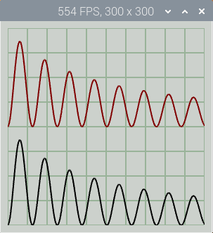
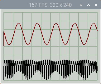
By default, 1000 points in two traces are plotted in a 300 x 300 pixel window; note the Frames Per Second (FPS) value in the title bar.

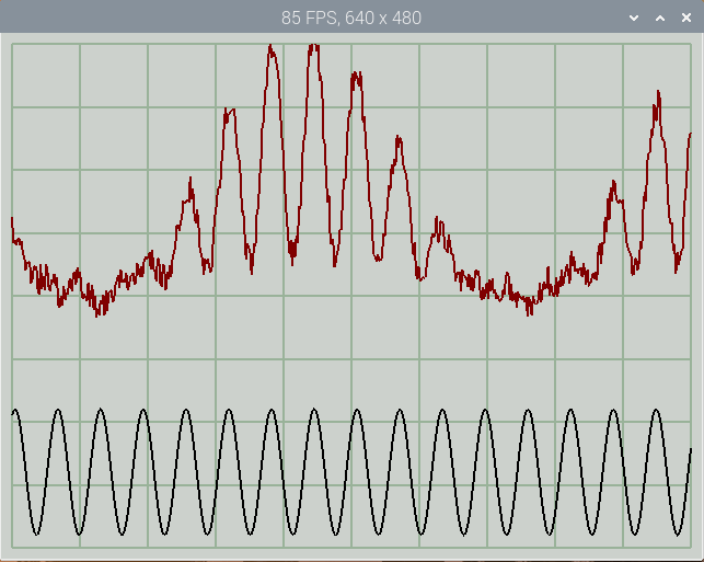
You can resize the window by specifying width & height in the standard X command-line format, e.g. for a 640 x 480 pixel window:

./rpi_opengl_graph -geometry 640x480

There is a simple console interface with 2 case-insensitive commands: ‘q’ to quit the application, and ‘p’ (or space-bar) to pause or resume the display updates.

My rpi_adc_stream application from a previous post can be used to supply the data, for example a single channel with 1000 points at 30k sample/s:

In one console:
   sudo ../dma/rpi_adc_stream -r 30000 -s /tmp/adc.fifo -i 1 -n 1000
In a second console:
  ./rpi_opengl_graph -geometry 1024x768 -i 1 -n 1000

The data source has to be run first, otherwise it won’t be detected by the graph utility.

If you don’t have access to this ADC, here is a simple Python program that generates 1000 samples in 2 channels, 50 times a second.

# Simple simulation of ADC feeding Linux FIFO

import math, time, os, signal, sys, random

fifo_name = "/tmp/adc.fifo"
ymax = 2.0
delay = 0.02
nchans = 2
npoints = 1000
running = True
fifo_fd = None

def remove(fname):
    if os.path.exists(fname):
        os.remove(fname)

def shutdown(sig=None, frame=None):
    print("\nClosing..")
    if fifo_fd:
        f.close()
    remove(fifo_name)
    sys.exit(0)

print("%u samples, %u channels, %3.0f S/s" % (npoints, nchans, npoints/delay))
remove(fifo_name)
data = npoints * [0]
n = 0;
signal.signal(signal.SIGINT, shutdown)
os.mkfifo(fifo_name)
try:
    f = open(fifo_name, "w")
except:
    running = False
while running:
    for c in range(0, npoints, nchans):
        data[c] = (math.sin((n*2 + c) / 10.0) + 1.2) * ymax / 4.0
        if nchans > 1:
            data[c+1] = (math.cos((n*2 + c) / 100.0) + 0.8) * data[c]
            data[c+1] += random.random() / 4.0
    n += 1
    s = ",".join([("%1.3f" % d) for d in data])
    try:
        f.write(s + "\n")
        f.flush()
    except:
        running = False
    sys.stdout.write('.')
    sys.stdout.flush()
    time.sleep(delay)
shutdown()

Run this script in one console, then the display application in another console, specifying a suitable window size, e.g.

./rpi_opengl_graph -geometry 640x480

The display shows two traces, one with added noise to illustrate the fast update rate.

rpi_opengl_graph display with adc_sim input

Copyright (c) Jeremy P Bentham 2020. Please credit this blog if you use the information or software in it.

Streaming analog data from a Raspberry Pi

Analog to Digital Converter (ADC) driver software usually captures a single block of samples; if a larger dataset (or continuous stream) is required, it can be very difficult to merge multiple blocks without leaving any gaps.

In this post I describe a utility that runs from the command-line, and performs continuous data capture to a Linux First In First Out (FIFO) buffer, that can be accessed by another Pi program, written in any language. The software also captures a microsecond time-stamp for each data block, that can be used to validate the timing, making sure there are no gaps.

To achieve this performance, I’m heavily reliant on Direct Memory Access (DMA) as described in a previous post; if you are a newcomer to the technique, I suggest you experiment with that code first, since it is much simpler.

ADC hardware

AB Electronics ADC DAC Zero on a Pi 3B

For this demonstration I’m using the ‘ADC-DAC Pi Zero’ from AB Electronics; despite the name, it is compatible with the full range of RPi boards. It uses an MCP3202 12-bit ADC with 2 analog inputs, measuring 0 to 3.3 volts at up to 60K samples per second. It also has 2 analog outputs from an MCP4822 DAC; I had planned to include these in the current software, but ran out of time – they may well feature in a future post.

As is common with mid-range ADC boards, it uses the Serial Peripheral Interface zero (SPI0) for data transfers. It has a 4-wire interface (plus ground) comprising transmit & receive data, a clock line, and Chip Enable zero (CE0).

ADC serial protocol

To get a sample from the ADC, it is necessary to drive the Chip Enable (CE) line low, clock in a command, clock out the data, and drive CE high. The SPI clock signal isn’t just used for data transmission, it also controls the internal logic of the ADC, so there is a limit on how fast it can be toggled; the data sheet is a bit vague on this subject (only specifying a limit of 1.8 MHz with 5V supply, and 0.9 MHz with 2.7V), so I’ve used a conservative value of 1 MHz. The data format is a 4-bit command, a null bit, and 12-bit response, making an awkward size of 17 bits. My software ignores the least-significant bit, so uses more convenient 16-bit transfers, with a maximum rate of 60K samples/sec. The command and response format is:

COMMAND:
  Start bit:                 1
  Single-ended mode          1
  Channel number             0 or 1
  M.S. bit first             1
  Dummy bits for response    0 0 0 0 0 0 0 0 0 0 0 0

RESPONSE:
  Undefined bits (floating)  x x x x
  Null bit                   0
  Data bits 11 to 0          x x x x x x x x x x x x

So the command for channel 0 is D0 hex, channel 1 is F0 hex. The following oscilloscope trace shows 2 transfers at 50,000 samples per second; you can see that the CE line goes low one clock cycle before the start of the transaction, and goes high on the last clock edge. This is because I’ve used the automatic-CE capability of the SPI interface, which provides very accurate timings.

ADC readings on a Pi Zero

The voltage is calculated by taking the value from the lower 11 bits, multiplying by the reference voltage, and dividing by the full-scale value, so 0x2AC * 3.3 / 2048 = 1.102 volts.

Raspberry Pi SPI

The SPI controller has the following 32-bit registers:

  • CS (control & status): configuration settings, and status information
  • FIFO (first-in-first-out): 16-word buffers for transmit & receive data
  • CLK (clock divisor): set the clock rate of the SPI interface
  • DLEN (data length): the transmit/receive length in bytes (see below)
  • LTOH (LOSSI output hold delay): not used
  • DC (DMA configuration): set the trigger levels for DMA data requests

The bit fields within these registers are described in the BCM2835 ARM Peripherals document available here, and the errata here; I’ll be concentrating on aspects that aren’t fully described in that document.

CS bits 0 & 1: select chip enable. The terms Chip Enable (CE) and Chip Select (CS) are used interchangeably to describe the hardware line that enables communication with the ADC or DAC chip, but CS is confusing as there is a CS (Control & Status) register as well, so I prefer to use CE. Bits 0 & 1 of that register control which CE line is used; the ADC is on CE0, and the DAC is on CE1.

CS bits 4 & 5: Tx and Rx FIFO clear. When debugging, it is quite common for there to be data left in the FIFOs, so it is a good idea to clear the FIFOs on startup.

CS bit 7: transfer active. When in DMA mode, set this bit to enable the SPI interface for data transfers. The transfer will start when there is data to be transmitted in the FIFO; after the specified length of data has been transferred, this bit will be cleared.

CS bit 8: DMAEN. This does not enable DMA, it just configures the SPI interface to be more DMA-friendly, as I’ll describe below. It isn’t necessary to use DMA when DMAEN is set; when trying to understand how this mode works, I used simple polled code.

CS bit 11: automatically deassert chip select. When set, the SPI interface can automatically frame each 16-bit transfer with the CE line; setting it low before the start, and high at the end, as shown in the oscilloscope trace above.

There is a confusing interaction between Transfer Active bit (TA), and the Data Length register (DLEN). Basically there are 2 very different ways of setting the data length at the start of a transfer:

  1. If TA is clear, the length (in bytes) must first be set in the DLEN register. Then TA is set, and the transaction will start when there is data in the transmit FIFO.
  2. If TA is set, the DLEN register is ignored. The length (in bytes) must first be written into the FIFO, together with some of the CS register settings, then the transfer will start when data is written to the transmit FIFO.

I generally use the first method, but either is workable providing you have a clear idea of the whether the transfer is active or not – don’t forget that it is automatically cleared when the length becomes zero.

An additional complication comes from the fact that DMA transfers and FIFO registers are 4 bytes wide, but we’re only doing 2-byte transfers to the ADC. The remaining 2 bytes aren’t automatically discarded; they stay in the FIFO to be used by the next transaction. It is possible to use this fact, and economise on memory by having 2 transmit words in one 4-byte memory location, but this can get really confusing (particularly with method 2) so I use a clear-FIFO command in each transfer to remove the extra. This means that the transmit & receive data only uses 16 bits in every 32-bit word.

SPI, PWM and DMA initialisation

To initialise the SPI & PWM controllers, we need to know what master clock frequency they are getting, in order to calculate the divisor values that’ll produce the required output frequencies. The frequencies (in MHz) depend on which Pi hardware version we’re using:

Version   PWM   SPI   REG_BASE     DMA channels used by OS
ZeroW     250   400   0x20000000   0, 2, 4, 6
Zero2     250   250   0x3F000000   0, 2, 3, 4, 6
1         250   250   0x20000000   0, 2, 4, 6
2         250   250   0x3F000000   0, 2, 4, 6
3         250   250   0x3F000000   0, 2, 4, 6
4 or 400  375   200   0xFE000000   2, 11, 12, 13, 14

The channel usage was determined by running my rpi_disp_dma utility, and the PWM & SPI clock values were checked using the rpi_adc_stream application in test mode, as described later in this post.

Sadly, this table isn’t telling the whole truth with regard to the values for SPI master clock. These are the values in normal operation, however if the CPU temperature is too high, its clock frequency is scaled back, and so is the SPI master clock. Mercifully the PWM frequency remains constant, so the sample rate of our code is unaffected, but as you’ll see from the oscilloscope trace above, if we’re running at 50K samples per second, there isn’t a lot of spare time, so if the SPI clock slows down, the transfers could fail to complete, causing garbage data and/or DMA timeouts.

This will only be a problem if you’re working close to the maximum sample rate, and if necessary, there are various workarounds you can use; for example, increase the SPI frequency, since the ADC does seem to tolerate values greater then 1 MHz, or fix the CPU clock frequency by changing the settings in /boot/config.txt.

The table also includes a list of active DMA channels, obtained by my rpi_disp_dma utility, as described later. Based on this result, I generally use channels 7, 8 & 9 in my code but of course there is no guarantee these will remain unused in any future OS release. If in doubt, run the utility for yourself.

Using DMA

The only way of getting ADC samples at accurately-controlled intervals is to use Direct Memory Access (DMA). Once set up, this acts completely independently of the CPU, transferring data to & from the SPI interface. We probably don’t want to run the ADC flat out, so need a method of triggering it after a specific time delay. In the absence of any hardware timers (surprisingly, the RPi CPU doesn’t have any conventional counter/timers) we’re using the Pulse Width Modulation (PWM) interface for timed triggering (which is generally known as ‘pacing’).

So we need to set up 3 DMA channels; one for transmit data, one for receive data, and one for pacing. I’ve tried to make the process of doing this as simple as possible, with a very clean structure. The DMA Control Blocks (CBs) and data must be in un-cached memory, as described in my previous post, so I’ve simplified the program steps to:

  1. Prepare the CBs and data in user memory.
  2. Copy the CBs and data across to uncached memory
  3. Start the DMA controllers
  4. Start the DMA pacing

To keep the organisation of the variables very clear, they are in a structure that can be overlaid onto both the user and the uncached memory. Here is the code for steps 1 and 2:

typedef struct {
    DMA_CB cbs[NUM_CBS];
    uint32_t samp_size, pwm_val, adc_csd, txd[2];
    volatile uint32_t usecs[2], states[2], rxd1[MAX_SAMPS], rxd2[MAX_SAMPS];
} ADC_DMA_DATA;

void adc_dma_init(MEM_MAP *mp, int nsamp, int single)
{
    ADC_DMA_DATA *dp=mp->virt;
    ADC_DMA_DATA dma_data = {
        .samp_size = 2, .pwm_val = pwm_range, .txd={0xd0, in_chans>1 ? 0xf0 : 0xd0},
        .adc_csd = SPI_TFR_ACT | SPI_AUTO_CS | SPI_DMA_EN | SPI_FIFO_CLR | ADC_CE_NUM,
        .usecs = {0, 0}, .states = {0, 0}, .rxd1 = {0}, .rxd2 = {0},
        .cbs = {
        // Rx input: read data from usec clock and SPI, into 2 ping-pong buffers
            {SPI_RX_TI, REG(usec_regs, USEC_TIME), MEM(mp, &dp->usecs[0]),  4, 0, CBS(1), 0}, // 0
            {SPI_RX_TI, REG(spi_regs, SPI_FIFO),   MEM(mp, dp->rxd1), nsamp*4, 0, CBS(2), 0}, // 1
            {SPI_RX_TI, REG(spi_regs, SPI_CS),     MEM(mp, &dp->states[0]), 4, 0, CBS(3), 0}, // 2
            {SPI_RX_TI, REG(usec_regs, USEC_TIME), MEM(mp, &dp->usecs[1]),  4, 0, CBS(4), 0}, // 3
            {SPI_RX_TI, REG(spi_regs, SPI_FIFO),   MEM(mp, dp->rxd2), nsamp*4, 0, CBS(5), 0}, // 4
            {SPI_RX_TI, REG(spi_regs, SPI_CS),     MEM(mp, &dp->states[1]), 4, 0, CBS(0), 0}, // 5
        // Tx output: 2 data writes to SPI for chan 0 & 1, or both chan 0
            {SPI_TX_TI, MEM(mp, dp->txd),          REG(spi_regs, SPI_FIFO), 8, 0, CBS(6), 0}, // 6
        // PWM ADC trigger: wait for PWM, set sample length, trigger SPI
            {PWM_TI,    MEM(mp, &dp->pwm_val),     REG(pwm_regs, PWM_FIF1), 4, 0, CBS(8), 0}, // 7
            {PWM_TI,    MEM(mp, &dp->samp_size),   REG(spi_regs, SPI_DLEN), 4, 0, CBS(9), 0}, // 8
            {PWM_TI,    MEM(mp, &dp->adc_csd),     REG(spi_regs, SPI_CS),   4, 0, CBS(7), 0}, // 9
        }
    };
    if (single)                                 // If single-shot, stop after first Rx block
        dma_data.cbs[2].next_cb = 0;
    memcpy(dp, &dma_data, sizeof(dma_data));    // Copy DMA data into uncached memory

The initialised values are assembled in dma_data, then copied into uncached memory at dp. The control blocks are at the start of the structure, to be sure they’re aligned to the nearest 32-byte boundary. Then there is the data to be transmitted, and some storage for the timestamps, that is marked as ‘volatile’ since it will be modified by DMA.

The format of a control block is:

  • Transfer Information (TI): address increment, trigger signal (data request), etc.
  • Source address
  • Destination address
  • Transfer length (in bytes)
  • Stride: skip unused values (not used)
  • Next Control Block: zero if last block
  • Debug: additional diagnostics

Looking at the first control block (CB 0) in detail:

#define SPI_RX_TI       (DMA_SRCE_DREQ | (DMA_SPI_RX_DREQ << 16) | DMA_WAIT_RESP | DMA_CB_DEST_INC)

{SPI_RX_TI, REG(usec_regs, USEC_TIME), MEM(mp, &dp->usecs[0]),  4, 0, CBS(1), 0}, // 0

Transfer info:       wait for data request from SPI receiver
Source address:      microsecond counter register
Destination address: memory
Transfer length:     4 bytes
Stride:              not used
Next control block:  CB 1
Debug:               not used

The source and destination addresses are more complex than usual, since they must be bus address values, created using a macro that takes a pointer to a block of mapped memory, and the offset within that block.

For this application, we need to keep re-transmitting the same bytes to request the data, but reception is in the form of long blocks of data; I’ve specified 2 blocks, that form a ‘ping-pong’ buffer, with the microsecond timestamp being stored at the start of each block, and a completion flag at the end. Ideally, the user code will be emptying one buffer while the other is being filled by DMA, but if the code is too slow, the overrun condition can be detected, and the data discarded.

Starting DMA

When we start the 3 DMA channels, they will all remain idle until the condition specified in TI is fulfilled:

    init_pwm(PWM_FREQ, pwm_range, PWM_VALUE);   // Initialise PWM, with DMA
    *REG32(pwm_regs, PWM_DMAC) = PWM_DMAC_ENAB | PWM_ENAB;
    *REG32(spi_regs, SPI_DC) = (8<<24) | (1<<16) | (8<<8) | 1;  // Set DMA priorities
    *REG32(spi_regs, SPI_CS) = SPI_FIFO_CLR;                    // Clear SPI FIFOs
    start_dma(mp, DMA_CHAN_C, &dp->cbs[6], 0);  // Start SPI Tx DMA
    start_dma(mp, DMA_CHAN_B, &dp->cbs[0], 0);  // Start SPI Rx DMA
    start_dma(mp, DMA_CHAN_A, &dp->cbs[7], 0);  // Start PWM DMA, for SPI trigger

To set the data-gathering in motion, we just enable PWM.

// Start ADC data acquisition
void adc_stream_start(void)
{
    start_pwm();
}

This sends a data request, which is fulfilled by DMA channel A (CB7), and nothing else happens; the SPI interface remains idle. However, on the next PWM timeout, CBS 8 & 9 are executed, which loads a value of 2 into the DLEN register, and sets the SPI transfer active. This triggers a request for Tx data from DMA channel C (CB6); when the first 2 bytes have been transferred, DMA channel B is triggered to store the microsecond timestamp (CB0), and the data (CB1). Since the transfer is no longer active, the DMA channels will all wait for their trigger signals, and the cycle will repeat, except that CB1 is storing the incoming ADC data in a single block.

Once the required number of samples have been received, CB2 sets a flag to indicate the buffer is full, then CB4 starts filling the other buffer.

Compiling and running the code

The C source code for the streaming application rpi_adc_stream and the DMA detection application rpi_disp_dma are on github here. You’ll also need the utility files rpi_dma_util.c and rpi_dma_util.h from the same directory.

Edit the top of rpi_dma_util.h to indicate which hardware version you are using (0 to 4, or 2 for the Zero2). The applications are compiled using a minimal command line:

gcc -Wall -o rpi_disp_dma rpi_disp_dma.c rpi_dma_utils.c
gcc -Wall -o rpi_adc_stream rpi_adc_stream.c rpi_dma_utils.c

You can add extra compiler options such as -O2 for code optimisation, but this isn’t really necessary.

Both of the utilities have to be run using ‘sudo’, as they require root privileges.

DMA channel scan

The DMA scan is run as follows:

Command:
  sudo ./rpi_disp_dma
Response (Pi ZeroW):
  DMA channels in use: 0 2 4 6

There is only one command line option, ‘-v’ for verbose operation, which prints out all the DMA register values.

By default, DMA_CHAN_A, B and C are defined in rpi_dma_utils.h as channels 7, 8 and 9, so should not conflict with those used by the OS.

ADC streaming

There are various command-line options, but it is suggested that you start by using the -t option to check the SPI and PWM interfaces are running correctly:

Command:
  sudo ./rpi_adc_stream -t
Response:
  RPi ADC streamer v0.20
  VC mem handle 5, phys 0xde50f000, virt 0xb6f5f000
  Testing 1.000 MHz SPI frequency:   1.000 MHz
  Testing   100 Hz  PWM frequency: 100.000 Hz
  Closing

A small error in the reading (e.g. 100.010 Hz) doesn’t indicate a fault, it is just due to the limited resolution of the timer that is making the measurement.

The command-line options are case-insensitive:

-F <num>    Output format, default 0. Set to 1 to enable microsecond timestamps.
-I <num>    Number of input channels, default 1. Set to 2 if both channels required.
-L          Lockstep mode. Only output streaming data when the Linux FIFO is empty.
-N <num>    Number of samples per block, default 1.
-R <num>    Sample rate, in samples per second, default 100.
-S <name>   Enable streaming mode, using the given FIFO name.
-T          Test mode
-V          Verbose mode. Enable hexadecimal data display.

Running the utility with no arguments will perform a single conversion on the first ADC channel (marked ‘IN1’):

Command:
  sudo ./rpi_adc_stream
Response:
  RPi ADC streamer v0.20
  VC mem handle 5, phys 0xde50f000, virt 0xb6fd1000
  SPI frequency 1000000 Hz
  ADC value 686 = 1.105V
  Closing

If the input isn’t connected to anything, you will get a random result; either short-circuit the input pins, or connect them to a known voltage source (less than 3.3V) to get a proper reading.

To stream the voltage values, it is necessary to specify the number of samples per block, the sample rate, and a Linux FIFO name; you can choose (almost) any name you like, but it is recommended to put the FIFO in the /tmp directory, e.g.

Command:
  sudo ./rpi_adc_stream -n 10 -r 20 -s /tmp/adc.fifo
Response:
  RPi ADC streamer v0.20
  VC mem handle 5, phys 0xde50f000, virt 0xb6f7e000
  Created FIFO '/tmp/adc.fifo'
  Streaming 10 samples per block at 20 S/s

The software is now waiting for another application to open the Linux FIFO, before it will start streaming. The FIFO is very similar to a conventional file, so some of the standard file utilities can be used, e.g. ‘cat’ to print the file. Open a second Linux console, and in it type:

Command:
  cat /tmp/adc.fifo
Response (with 1.1V on ADC 'IN1'):
  1.102,1.104,1.104,1.102,1.104,1.104,1.110,1.104,1.102,1.102
  1.105,1.104,1.104,1.104,1.105,1.102,1.102,1.104,1.104,1.104
  ..and so on, at 2 blocks per second..

Hit ctrl-C to stop this command, and you’ll see that the streamer can detect that there is nothing reading the FIFO, so reports ‘stopped streaming’, though it does continue to fetch data using DMA, since this has minimal impact on any other applications.

You’ll note that it hasn’t been necessary to run the data display command using ‘sudo’; it works fine from a normal user account. It is important to limit the amount of code that has to run with root privileges, and the Linux FIFO interface is a handy way of achieving this.

There is a ‘-f’ format option, that controls the way the data is output. Currently there is only one possibility ‘-f 1’ which enables a microsecond timestamp on each block of data, e.g.

Command in console 1:
  sudo ./rpi_adc_stream -n 1 -r 10 -f 1 -s /tmp/adc.fifo
Response:
  Streaming 1 samples per block at 10 S/s

Command in console 2:
  cat /tmp/adc.fifo
Response in console 2 (with 1.1 volt input):
  0,1.102
  100000,1.104
  200000,1.102
  300001,1.105
  400001,1.104
  ..and so on, at 10 lines per second

The timestamp started at zero, then incremented by 100,000 microseconds every block. It is a 32-bit number, so if you want to measure times longer than 7 minutes, you will need to detect when the value has wrapped around.

If 2 input channels are enabled using ‘-i 2’, then the overall sample rate remains unchanged, each channel has half the samples. In the following example, I’ve also enabled verbose mode, to see the ADC binary data:

Command in console 1:
  sudo ./rpi_adc_stream -n 2 -i 2 -r 10 -f 1 -s /tmp/adc.fifo -v
Response in console 1:
  Streaming 2 samples per block at 10 S/s
Response when streaming starts:
  Started streaming to FIFO '/tmp/adc.fifo'
  F2 AD 00 00 F0 01 00 00
  F2 AE 00 00 F0 01 00 00
  F2 AE 00 00 F0 01 00 00
  F2 AE 00 00 F0 00 00 00
  ..and so on..

Command in console 2:
  cat /tmp/adc.fifo
Response in console 2 (IN1 is 1.1 volts, IN2 is zero):
  1.104,0.002
  1.105,0.002
  1.105,0.002
  1.105,0.000
  ..and so on..

Displaying streaming data

It’d be nice to view the streaming data in a continually-updated graph, similar to an oscilloscope display, but surprisingly few graphing utilities can handle a continuous flow of data – or they can only handle it at a very low rate.

Here are a few graphing utilities I’ve tried; they perform reasonably well on fast hardware, but struggle to maintain a good-quality graph on slower boards such as the Pi Zero – there is no problem with the data acquisition, it is just that the graphical display is very demanding.

Trend display

There is a Linux utility called ‘trend’, that can dynamically plot streaming data.

Trend display of a 50 Hz analog signal, 5000 samples per second

It has a wide range of options, and keyboard shortcuts, that I haven’t yet explored. The above graph was generated on a Pi 4 using the following command in one console:

sudo ./rpi_adc_stream -n 1 -l -r 5000 -s /tmp/adc.fifo

Then in a second console, the application is installed and run:

sudo apt install trend
cat /tmp/adc.fifo | trend -A f0f0f0 -I ff0000 -E 0 -s -v - 1200 600

This application is quite demanding on CPU resources, so if you are using a Pi 3, you’ll probably need to drop the sample rate to 2000.

Termeter display

Termeter is a really useful text-based dynamic display utility, written in the Go language.

You may wonder why I’m using a text-based console application to produce a graph, but it has two key advantages; it is very fast, and works on any Pi console. So if you are running the Pi ‘headless’ (i.e. remotely, with no local display) and you want to look your streaming data, you can run termeter on a remote console (e.g. ‘putty’ on windows) without the complexity of setting up an X display server.

It is installed using:

cd ~
sudo apt install golang
go get github.com/atsaki/termeter/cmd/termeter

The above data (1 sample per block, 5000 samples per second) was generated on a Pi 4 by running in one console:

sudo ./rpi_adc_stream -n 1 -r 5000 -s /tmp/adc.fifo

Then the display is started in a second console:

cat /tmp/adc.fifo | ~/go/bin/termeter

On a Pi 3, you might have to drop the sample rate to 2000, and even further on a Pi Zero.

Plotting in Python

Python plot of streaming data

Here is a very simple example that uses NumPy and Matplotlib to create a dynamically-updated graph of ADC data (a 10 Hz sine wave, at 200 samples per second, on a Pi 4). In one terminal, the data is generated by running:

sudo ./rpi_adc_stream -n 100 -r 200 -l -s /tmp/adc.fifo

Then run the following program in a second terminal (assuming you’ve installed Matplotlib and NumPy):

import numpy as np
from matplotlib import pyplot, animation

fifo_name = "/tmp/adc.fifo"
npoints  = 100
interval = 500
xlim     = (0, 1)
ylim     = (0, 3.5)

fifo = open(fifo_name, "r")
fig = pyplot.figure()
ax = pyplot.axes(xlim=xlim, ylim=ylim)
line, = ax.plot([], [], lw=1)

def init():
    line.set_data([], [])
    return line,

def animate(i):
    x = np.linspace(0, 1, npoints)
    y = np.fromstring(fifo.readline(), sep=',')
    line.set_data(x, y)
    return line,

anim = animation.FuncAnimation(fig, animate, init_func=init,
                               frames=npoints, interval=interval, blit=True)
pyplot.show()

The ‘readline’ function fetches a single line of comma-delimited data, which ‘fromstring’ converts to a NumPy array.

The ‘animate’ function is used to continuously refresh the graph, however this approach is only suitable for low update rates; the time taken to do the plot is quite significant, and there is an inherent conflict between the data rate set by the streamer, and the display rate set by the animation, causing the display to stall, especially on a single-core Pi Zero. A multi-threaded program is needed to coordinate the display updates with the incoming data.

Update

The display problem has been solved by creating a fast oscilloscope-type viewer for the streaming data, using OpenGL.

WebGL oscilloscope display

Full details and source code are here, and there is a WebGL version that works remotely in a browser here.

Copyright (c) Jeremy P Bentham 2020. Please credit this blog if you use the information or software in it.