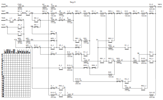
There are plenty of circuit simulators available, that give detailed analysis of circuits with capacitors, inductors and semiconductors, and these can be used to simulate a purely resistive circuit (such as a 1938 ‘Q’ stock traction control, as shown above) but they lack the flexibility to show the remarkable 19 state-changes that occur when the train accelerates. Furthermore, the simulation process is quite complex, and it is difficult to understand how the simulator obtains its results.
So I’ve created a simple simulator in Python, that solves DC resistive circuits, and is capable of being embedded as a component in other applications; its output can even be used to draw an animated sequence of circuit diagrams, annotated with the voltages and currents flowing through each component.
Voltage or current?
When attempting to analyse a circuit, there are two methods that can be used: Kirchhoff’s first (‘current’) law, or second (‘voltage’) law. There are plenty of descriptions of these laws online, but in brief they say that the sum of currents at a point, or voltages in a loop, must be zero. Taking the following simple circuit as an example:
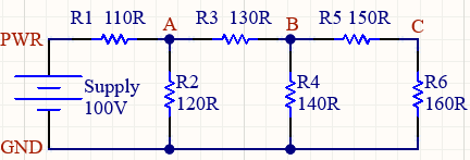
This has a 100 volt supply, and six resistors with values between 110 and 160 ohms. The junctions between the resistors have been labelled with letters A to C, with power & ground lines abbreviated to ‘PWR’ and ‘GND’.
If we were to use the second law, then we first have to identify the loops in the circuit, for example the battery R1 & R2, then R2 R3 & R4, and so on. This is easy to do in such a simple circuit, but the analysis can become quite complicated when the circuit is more realistic.
In contrast, using the first law is simpler to implement, the node ‘A’ gets current from R1 R2 & R3, ‘B’ from R3 R4 & R5, and so on.
So for simplicity, I’ll be using the first (‘current’) law. To calculate the voltage at each point, the effective resistance needs to be known, which is the parallel resistance of the resistors connected to that point, e.g. point ‘A’ is connected to R1, R2 & R3, so the effective resistance for that point is 1 / ((1/R1) + (1/R2) + (1/R3)) = 39.814 ohms.
Parts
This presumes we have entered the supply and resistances into the program, but how should this be done? An electronics CAD program can generate a ‘netlist’ which details the connections between components, but this can be quite vendor-specific, and generally does not include component values, which are documented in a separate parts list. So to avoid the complexities of file formats, the components and their connections are entered as instantiations of Python classes, e.g.
parts = (
    Res("R1",   ['PWR', 'a'], 110.0),
    Res("R2",   ['a', 'GND'], 120.0),
    Res("R3",   ['a', 'b'],   130.0),
    Res("R4",   ['b', 'GND'], 140.0),
    Res("R5",   ['b', 'c'],   150.0),
    Res("R6",   ['c', 'GND'], 160.0)
)
A class is used to define a generic part, with the resistor subclass called ‘Res’. This is defined with a name, array of node names, and resistance:
class Part(object):
    def __init__(self, name, nodenames, res=0.0, posn=None):
        self.name, self.nodenames = name, nodenames
        self.res, self.posn, self.typ = res, posn, None

class Res(Part):
    def __init__(self, name, nodenames, res=0.0, posn=None):
        super(Res, self).__init__(name, nodenames, res, posn)
        self.typ = "Res"
These classes permit other parts to be constructed, as subclasses of ‘Part’. The ‘type’ field (called ‘typ’) can house a string that is used to distinguish between parts. The ‘position’ field (called ‘posn’) can optionally house the position of the part on a circuit diagram; it is unused in this example.
Nodes
The nodes have been lettered A to C on the circuit diagram, with PWR for power, and GND for ground. The ‘part’ class definitions contain all the information we need to derive a list of nodes, so there is no need to manually enter this information. A function can be used extract the nodes from the list of parts, and store them in an array of class instances, see the ‘circuit’ class below.
class Node():
    maxnum = 0
    def __init__(self, name, volts=0.0):
        self.name, self.volts = name, volts
        self.conductance = 0.0
        self.parts = []
        self.num = Node.maxnum
        self.checked = False
        Node.maxnum += 1
Each node is attached to one or more parts, so the node has an array to store this information, so it possible to identify which parts are linked to a node.
The ‘conductance’ of a node is the inverse of its resistance, and reflects the parallel resistance of all the linked parts. This is easier to compute on-the-fly than parallel resistance, so for example node A has the parallel resistance of R1, R2 and R3, so R = 1 / (1/R1 + 1/R2 + 1/R3). If instead we use conductances, G = G1 + G2 + G3, where G1 = 1/R1, G2 = 1/R2, G3=1/R3.
The ‘num’ and ‘maxnum’ field are used to generate a unique number for each node. This is necessary because the ‘numpy’ numerical package works with arrays that have numerical dimensions, unlike the usual Python arrays which can use numerical values or strings.
The ‘checked’ field is used to raise an error if a node is completely isolated from all other nodes, as the array-creation code will fail if that is the case. It is acceptable to have a part with only one connection, but parts with zero ongoing connections will trigger an error.
Power and ground are special nodes, that are defined using arrays, in case we need to have multiple power or ground connections. The voltage is also specified using a ‘supply’ variable:
    SUPPLY  = 100
    GROUNDS = ["GND"]
    POWERS  = ["PWR"]
Circuit
This class encapsulates the parts, power & ground, and provides functions to manipulate that information, e.g. extracting the list of nodes from the list of parts:
class Circuit(object):
    def __init__(self, parts, supply, grounds=["GND"], powers=["PWR"]):
        self.parts = {}
        for part in parts:
            if part.name in self.parts:
                print("Duplicate part: %s" % part.name)
                break
            self.parts[part.name] = part
        self.supply, self.grounds, self.powers = supply, grounds, powers

    def get_nodes(self):
        nodes = {}
        Node.maxnum = 0
        for part in self.parts.values():
            for nodename in part.nodenames:
                if nodename not in nodes:
                    node = Node(nodename)
                    nodes[node.name] = node
                else:
                    node = nodes[nodename]
                if part.res > 0:
                    node.conductance += 1.0 / part.res
                node.parts.append(part)
        self.nodes = dict(sorted(nodes.items()))
Simulation
The resistor network can be expressed as a set of simultaneous equations; solving these equations gives us the voltages of the nodes. The ‘circuit’ class contains the code to do the simulation, but first we can demonstrate the calculation process by doing the steps manually, with a little bit of help from the Python ‘numpy’ numeric calculation library to do the array arithmetic:
import numpy as np

# Pretty print a 1-dimensional array
def vector_str(v):
    return " ".join(["%10.6f" % val for val in v])

# ASCII version of circuit diagram
#  P      a      b      c
#  |--R1-----R3-----R5--|
#         |      |      |
#         R2     R4     R6
# GND     |      |      |
#  |--------------------|

# Resistor definitions, and supply voltage
R1 = 110; R2 = 120; R3 = 130; R4 = 140
R5 = 150; R6 = 160; VIN = 100

# Calculation of effective resistance of each node
Ra = 1 / (1/R1 + 1/R2 + 1/R3)
Rb = 1 / (1/R3 + 1/R4 + 1/R5)
Rc = 1 / (1/R5 + 1/R6)
Rp = R1

# Ohms law equations for nodes a, b, c and p (power)
# Va = (Vp/R1 + Vb/R3) * Ra
# Vb = (Va/R3 + Vc/R5) * Rb
# Vc = (Vb/R5)         * Rc
# Vp = VIN

# Rearrange equations so constant on left-hand side
# 0    = -Va       + Vb*Ra/R3            + Vp*Ra/R1
# 0    =  Va*Rb/R3 - Vb       + Vc*Rb/R5
# 0    =             Vb*Rc/R5 - Vc
# -VIN =                                 - Vp

# Create arrays
#     Va     Vb     Vc     Vp
x = [[-1,    Ra/R3, 0,     Ra/R1],
     [Rb/R3, -1,    Rb/R5, 0    ],
     [0,     Rc/R5, -1,    0    ],
     [0,     0,     0,     -1   ]]

y =  [0,     0,     0,     -VIN]

# Solve the equations
volts = np.linalg.inv(x).dot(y)
# or volts = np.linalg.solve(x, y)
print(vector_str(volts))

# Calculated voltages on nodes a, b, c, p
# 41.624400  17.728155   9.150015 100.000000
The above example code can be run standalone to illustrate the steps involved in the simulation.
The real simulation code (shown below) iterates through the list of nodes, scanning the parts connected to that node, and preparing the arrays that hold the equation data. Once they are complete, some simple matrix arithmetic gives the voltages at each of the nodes.
    MAX_RES = 1e9
    def simulate(self):
        # Create arrays
        n = len(self.nodes)
        array  = np.zeros([n, n])
        vector = np.zeros(n)

        # Iterate across nodes
        for node in self.nodes.values():
            # Initialise matrix diagonal
            array[node.num][node.num] = -1

            # Iterate across parts connected to node
            for part in node.parts:
                # Skip if one of the nodes is ground
                if not (set(self.grounds) & set(part.nodenames)):

                    # Iterate across nodes connected to part
                    for nodename in part.nodenames:
                        nextnode = self.nodes[nodename]
                        # Check for a power node
                        if node.name in self.powers:
                            vector[node.num] = -self.supply
                        # If part is not already referenced..
                        elif node.name != nextnode.name and part.res <= MAX_RES:
                            # Get current using ohms law
                            val = 1.0/(node.conductance * part.res)
                            array[node.num][nextnode.num] = val
        # Solve simultaneous equations
        voltages = np.linalg.solve(array, vector)
        for node in self.nodes.values():
            node.volts = voltages[node.num]
One point that deserves explanation is the use of MAX_RES, which gives a maximum resistance, above which the node is ignored. This is necessary because the array arithmetic has a limited dynamic range; if that is exceeded, the voltage calculation can be inaccurate.
Running the code
The quicksim.py source file is available on github here
It is compatible with Python 3; the only dependency is the numpy mathematics package, which is used for matrix calculation.
As standard, it simulates the minimal resistor network described above.
    SUPPLY  = 100
    GROUNDS = ["GND"]
    POWERS  = ["PWR"]

    parts = (
        Res("R1",   ['PWR', 'a'], 110.0),
        Res("R2",   ['a', 'GND'], 120.0),
        Res("R3",   ['a',   'b'], 130.0),
        Res("R4",   ['b', 'GND'], 140.0),
        Res("R5",   ['b',   'c'], 150.0),
        Res("R6",   ['c', 'GND'], 160.0))
The supply voltage can be changed as required; since the circuit is linear, this will just change the node voltages in proportion. The power and ground connections are implemented as arrays, so there can potentially be multiple power and ground connections. The resistors are defined with a name, two node connections, and a resistance. Running the simulation produces a verbose output, showing the part & node definitions:
cct = Circuit(parts, SUPPLY, GROUNDS, POWERS)
    cct.get_nodes()
    fails = cct.check_nodes()
    if fails:
        print("\nFloating nodes: " + fails)
    else:
        cct.simulate()
        print("Parts\n" + cct.list_parts())
        print("Nodes\n" + cct.list_nodes())
        print("Voltages\n" + cct.list_voltages())
The check for floating nodes will detect those that are completely isolated from power or ground; if these nodes are not caught, they will cause the matrix arithmetic to fail.
The console output lists the parts, nodes, and node voltages:
Parts
Part R1 (nodes PWR a) res 110.000
Part R2 (nodes a GND) res 120.000
Part R3 (nodes a b) res 130.000
Part R4 (nodes b GND) res 140.000
Part R5 (nodes b c) res 150.000
Part R6 (nodes c GND) res 160.000

Nodes
Node GND (parts R2 R4 R6) par_res 46.027
Node PWR (parts R1) par_res 110.000
Node a   (parts R1 R2 R3) par_res 39.814
Node b   (parts R3 R4 R5) par_res 46.508
Node c   (parts R5 R6) par_res 77.419

Voltages
Node PWR: 100.000V
Node   a:  41.624V
Node   b:  17.728V
Node   c:   9.150V
In future posts, I will show how this simulation can be extended to include dynamic components (such as electromagnetic relays) and can even be used to create animated display of a 1938-vintage circuit that controls a London underground train. More to follow…
Copyright (c) Jeremy P Bentham 2026. Please credit this blog if you use the information or software in it.
