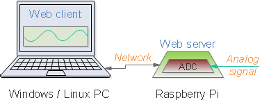
In a previous post, I gathered analog data on the Raspberry Pi, and used OpenGL to plot a fast oscilloscope-type graphic. However, in many cases it is inconvenient to have a local display; it would be much better to send the data over the network, to be displayed remotely.
Separating the data-gathering from the data-display has many other advantages. Modern PCs can draw graphics at very high speed, so offloading this task from the Pi makes a lot of sense; it is also possible to view the real-time image on a tablet or mobile phone, removing the need for bulky equipment and cabling.

If you want to display logic waveforms instead of analogue traces, see my other post.
WebGL programming
WebGL works within a Web browser, to provide hardware-accelerated graphics, similar to OpenGL. It is essentially OpenGL ES, with a Javascript wrapper for compatibility with other browser code.
If you are a newcomer to OpenGL, I suggest you read one of the many tutorials on the Web; there are also ‘live’ interactive sites, where you can experiment with code, and immediately see the result.
There are two fundamental approaches to using WebGL graphics; you can treat it as a simple graphics card, and issue sequential commands to individually draw the display items you want, but this approach can be quite slow, as the repated handovers between Javascript and OpenGL take a significant amount of time.
Alternatively, you can pre-prepare the object to be drawn as an array of 3D data points (known as ‘vertex attributes’), then issue a single call to OpenGL to render those points. This is much faster, as the graphics hardware can work at top speed processing the points.

Each vertex attribute can have multiple dimensions; I’m using 3 dimensions for each point. The x and y values are normalised to +/- 1.0, so the bottom left corner of the graph is -1, -1, and the top right is +1.0, +1.0. The shaders have a very powerful matrix-arithmetic capability, so it is easy to transform these values into a user-defined scale, but I’ve found this can be very confusing, so I’ve kept the normalised defaults.
The z-value is used to indicate which trace is being drawn; the background grid is z = zero, the first trace is z = 1.0, and so on.
The vertex shader must be instructed what to do with the array of vertices. My previous Raspberry Pi code used ‘strip’ mode (GL_LINE_STRIP), which meant that the vertices form a single continuous polyline, the end of one line segment being used as the start of the next. This had the advantage of minimising the amount of data needed, but meant that I had to perform some z-value tricks to handle the transition from the end of one trace to the start of the next.
To avoid that problem, in this project I’ve used ‘line’ mode (gl.LINES) whereby each line is drawn individually, with a pair of vertices to mark its start & end. This almost doubles the amount of data we have to send to the shader, but does simplify the code.
WebGL versions
Modern browsers support can support WebGL version 1.0 and 2.0. The former is based on OpenGL ES 2.0, the latter OpenGL ES 3.0. To add to the confusion, the GLSL shader language is version 1 for OpenGL ES 2, and version 2 for OpenGL ES 3.
Why does this matter? Unfortunately there are significant differences between the two shader language versions; you can’t create a single source-file that works with both. Many of the examples on the Web don’t specify which version they are targeting, but it is quite easy to tell: if some variables are defined using ‘in’ and ‘out’, then the language is GLSL v2, e.g.
// GLSL v2 definitions:
  in vec3 a_coords;
  out vec4 v_colour;

// GLSL v1 definitions:
  attribute vec3 a_coords;
  varying vec4 v_colour;
I have provided both versions, with a boolean Javascript constant (WEBGL2) to switch between them.
Shader programming
The core of our application is the shader code, that processes the attributes. We are using two shaders; one to convert the vertices into ‘fragment’ data, and the other to convert the fragments into pixels. Since the shader programs are quite short, they can be included as ‘template literal’ strings in the Javascript code. These begin and end with a back-tick (instead of a single or double quote character) and can have multiple lines, with the possibility of variable substitution. The vertex shader code is
vert_code = `#version 300 es
    #define MAX_CHANS ${MAX_CHANS}
    in vec3 a_coords;
    out vec4 v_colour;
    uniform vec4 u_colours[MAX_CHANS];
    uniform vec2 u_scoffs[MAX_CHANS];
    vec2 scoff;
    void main(void) {
        int zint = int(a_coords.z);
        scoff = u_scoffs[zint];
        gl_Position = vec4(a_coords.x, a_coords.y*scoff.x + scoff.y, 0, 1);
        v_colour = u_colours[zint];
    }`;
The 300 ES version definition must be on the first line, or it will be rejected.
The strange-looking MAX_CHANS definition takes the value of a Javascript constant, and creates a matching GLSL definition.
The z-value of each vertex is used to determine the drawing colour by indexing into a ‘uniform’ array, i.e. an array that has been preset in advance by the Javascript code. The z-value is also used to determine the y-value scale and offset (‘scoff’), obtained from another uniform array. So the magnitude and offset of each trace can be individually controlled, by changing the constants loaded into the ‘scoff’ array.
The fragment shader doesn’t do much; it just copies the colour of the fragment into the colour of the pixel:
frag_code = `#version 300 es
    precision mediump float;
    in vec4 v_colour;
    out vec4 o_colour;
    void main() {
        o_colour = v_colour;
    }`;
These programs need to be compiled before use, and there is some simple Javascript code to do this, but that raises the question: if there is an error, how is it displayed, since we’re in a browser? I’ve taken an easy way out and thrown an exception:
// Compile a shader
function compile_shader(typ, source) {
    var s = gl.createShader(typ);
    gl.shaderSource(s, source);
    gl.compileShader(s);
    if (!gl.getShaderParameter(s, gl.COMPILE_STATUS))
        throw "Could not compile " +
              (typ==gl.VERTEX_SHADER ? "vertex" : "fragment") +
              " shader:\n\n"+gl.getShaderInfoLog(s);
    return(s);
}
The error messages are sometimes a bit simplistic, and you may need to be a bit creative when working out what is wrong, so it is recommended that you do frequent re-compiles, to quickly identify any issues.
The shader code and Javascript is all in a single HTML file, that can be directly loaded into a browser from the filesystem; on startup, it displays 2 channels of static test data, to prove that WebGL is working.

HTML
The GLSL shader code, and the associated Javascript program, are encapsulated in a single HTML file, webgl_graphics.html. It defines the ‘canvas’ area that will house the the WebGL graphic, and some buttons and selectors for the user to control the display, with a preformatted text line to display status information.
  <canvas id = "graph_canvas"></canvas>
  <button id="single_btn"   onclick="run_single(this)">Single</button>
  <button id="run_stop_btn" onclick="run_stop(this)"  >Run</button>
  <select id="sel_nchans" onchange="sel_nchans()"></select>
  <select id="sel_srce"   onchange="sel_srce()"  ></select>
  <pre id="status" style="font-size: 14px; margin: 8px"></pre>
I’ve kept the HTML simple, since the primary focus of this project is to demonstrate the high-speed graphics; there is plenty of scope for adding decoration, style sheets etc. to make a better-looking display.
Data acquisition
The Javascript program must repeatedly load in the data to be displayed, to create an animated graphic. There are security safeguards on the extent to which a browser can load files from a user’s hard disk; it is much easier if the files are loaded from a Web server. So I’m running a Python-based Web server (‘cherrypy’) to provide the HTML & data files. This works equally well on a Windows or Linux PC, as on a Raspberry Pi, so it is possible to test the WebGL rendering on any convenient machine, using simulated data.
In a previous post, I used DMA to stream data in from an analog-to-digital converter (ADC); the output is comma-delimited (CSV) data, sent to a Linux first-in-first-out (FIFO) buffer. There is a single text line, containing floating-point text strings, with interleaved channels, so if there are 2 channels, and channel 1 has a value floating around zero, channel 2 has a value around 1, then the data might look like:
0.000,1.000,0.001,1.000,0.000,1.001 ..and so on until..<LF>
There is an easy way to load in this data using Javascript:
    // Decode CSV string into floating-point array
    function csv_decode(s) {
        data = s.trim().split(',');
        return data.map(x => parseFloat(x));
    }
For simplicity, it is assumed that there is no whitespace padding between the values; if the file has been generated by an external application (e.g. spreadsheet) some extra string processing will be needed.
The total number of data values is split between the channels, so if there are 1000 samples and 2 channels, each channel has 500 samples.
Web server
The cherrypy Web server is Python-based, and is easy to install. We need to provide a small Python configuration program, which has a class definition, with methods for the resources that are provided, for example:
# Oscilloscope-type ADC data display
class Grapher(object):

    # Index: show oscilloscope display
    @cherrypy.expose
    def index(self):
        return cherrypy.lib.static.serve_file(directory + "/webgl_graph.html")

if __name__ == '__main__':
    cherrypy.config.update({"server.socket_port": portnum, "server.socket_host": "0.0.0.0"})
    conf = {
        '/': {
            'tools.staticdir.root': os.path.abspath(os.getcwd())
        }
    }
    cherrypy.quickstart(Grapher(), '/', conf)
The default index page is defined as webgl_graph.html in the current directory, and the socket_host definition allows that page to be accessed by any system on the network.
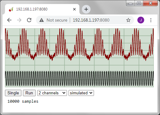
When this page is loaded from the Web server, it shows a simulated 2-channel display, and the status line reports the address and port number of the server.

Hitting the ‘single’ button will load 1000 simulated samples in 2 channels from /sim. The server code is:
    @cherrypy.expose
    def sim(self):
        global nresults
        cherrypy.response.headers['Content-Type'] = 'text/plain'
        data = npoints * [0]
        for c in range(0, npoints, nchans):
            data[c] = (math.sin((nresults*2 + c) / 20.0) + 1.2) * ymax / 4.0
            if nchans > 1:
                data[c+1] = (math.cos((nresults*2 + c) / 200.0) + 0.8) * data[c]
                data[c+1] += random.random() / 4.0
        nresults += 1
        rsp = ",".join([("%1.3f" % d) for d in data])
        return rsp
The lower channel is a pure sine wave, the upper is amplitude-modulated with added random noise, resulting in the following display:
The above tests will work with the web server & client running on any Linux or Windows PC. Loading real-time data from a hardware source (such as an ADC) is done using a Linux FIFO; the Javascript code is the same as reading from a file, but read cycle will produce new data each time:
    # FIFO data source
    @cherrypy.expose
    def fifo(self):
        cherrypy.response.headers['Content-Type'] = 'text/plain'
        try:
            f = open(fifo_name, "r")
            rsp = f.readline()
            f.close()
        except:
            rsp = "No data"
        return rsp
Running the code
Install the cherrypy server using:
# For Python 2
pip install cherrypy
# ..or for Python 3 on the Raspberry Pi
pip3 install cherrypy
Fetch the files adc_server.py and webgl_graph.html from github and load them into any spare directory. Run the server file using Python or Python3, and point your browser at the port 8080 of the server, e.g. 192.168.1.197:8080.
If all is well you should see the displays I’ve given above. If access is denied, you may have a firewall issue; if the HTML content is displayed, but the WebGL content isn’t, then check that WebGL is available on the browser, and perhaps set the Javascript WEBGL2 variable false, in order to try using version 1.
On the Raspberry Pi, my previous ADC streaming project can be used to feed real-time data into the FIFO, for example using the following command-line in one console:
# Stream 1000 samples from 2 ADC channels, 10000 samples/sec
sudo rpi_adc_stream -r 10000 -s /tmp/adc.fifo -n 1000 -i 2
Then run the Web server in a second console. If ADC channel 1 is fed with a modulated 1 kHz signal, and channel 2 is the 100 Hz sine-wave modulation, the display might look like:

The data transfer method (continuously re-reading a file on the server) isn’t the most efficient, and does impose an upper limit on the rate at which data can be fetched from the Raspberry Pi. It would probably be better to use an alternative technique such as WebSockets, as I’ve previously explored here.
Copyright (c) Jeremy P Bentham 2021. Please credit this blog if you use the information or software in it.
