Drawing graphics in browser-friendly SVG, with Javascript animation
My previous attempt at real-time graphics involved direct-drawing the shapes using Python and PyQt. This works well for a standalone system, but is less useful in the current world of ‘everything-on-a-browser’. To make the graphics Web-friendly, there is a choice; either create an animated bitmap (e.g. GIF, PNG or JPEG) or use vector graphics (SVG).
Vector graphics have various advantages; not just that they can be resized without degradation (pixellation) but also that they can preserve some of the structural characteristics of the image that is being animated. For example, we can draw a detailed circuit diagram complete with voltage and current measurements, and if it is too large to display in a browser screen, the user can zoom out to get the big picture, then zoom in to see the data in a specific area; the components will always appear well-drawn, no matter what scale is used.


If the components are drawn sensibly they can easily be annotated & animated to reflect the current data values. Unfortunately, although most graphics packages can export SVG, very few preserve the underlying structure of the parts. For example, the above circuit diagram was originally exported from Visio as an 800K file, filled with tiny vector & text fragments, that were very difficult to relate back to the original components. The final version, created by a Python program from a netlist, was 33KB in size, and much easier to animate.
I certainly wouldn’t give up on the idea of animating pre-existing circuit diagrams, but for the purposes of this blog, am taking the easy way out, and creating the graphics from scratch in Python. Also, it is quite a big step to create & animate a full circuit diagram in one go, so I’ll start with something much simpler, a 7-segment digital clock.

This will involve Python, SVG, style sheets and even a smattering of Javascript, so is complicated enough for starters. If you are going to do a lot of graphical manipulation, it is well worth reading the SVG specification.
svgwrite
My code is compatible with Python 2.7 or 3.x, you just need to install the ‘svgwrite’ package using pip or pip3.
As its name suggests, svgwrite is a relatively slim wrapper that simplifies the task of writing SVG files, for example:
# Create simple SVG
import svgwrite
FILENAME      = "simple.svg"
WIDTH, HEIGHT = 250, 150

dwg = svgwrite.Drawing(FILENAME, (WIDTH, HEIGHT))
dwg.add(dwg.rect((0,0),
                 (WIDTH-1,HEIGHT-1),
                 stroke="red",
                 fill="none"))
dwg.add(dwg.line((0,0),
                 (WIDTH-1,HEIGHT-1),
                 stroke="green",
                 stroke_width=8))
dwg.add(dwg.circle((WIDTH/2,HEIGHT/2),
                   HEIGHT/2,
                   stroke_width=3,
                   stroke="salmon",
                   fill="moccasin"))
dwg.add(dwg.circle((WIDTH/2,HEIGHT/2),
                   HEIGHT/3,
                   stroke_width=3,
                   stroke="salmon",
                   fill="moccasin"))
dwg.save()
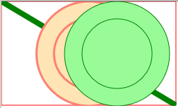
If the resulting SVG file is dragged into a browser, it looks like:

There are various points to note (apart from the author’s strange colour choices):
- The origin (x=0, y=0) is in the top left corner
- Coordinates are specified as (x,y) tuples
- The order of drawing is significant: earlier objects may be obscured by later
- Lines outside the drawing area are clipped
- To eliminate fill, you have to use ‘fill=”none”‘, rather than the more Pythonic ‘fill=None’
It is instructive to view the resulting file in a text editor; after the namespace boilerplate, there is a close match with the Python code:
<?xml version="1.0" encoding="utf-8" ?>
<svg baseProfile="full" height="150" version="1.1" width="250"
 xmlns="http://www.w3.org/2000/svg"
 xmlns:ev="http://www.w3.org/2001/xml-events"
 xmlns:xlink="http://www.w3.org/1999/xlink">
 <defs />
 <rect fill="none" height="149" stroke="red" width="249" x="0" y="0" />
 <line stroke="green" stroke-width="8" x1="0" x2="249" y1="0" y2="149" />
 <circle cx="125" cy="75" fill="moccasin" r="75" stroke="salmon" stroke-width="3" />
 <circle cx="125" cy="75" fill="moccasin" r="50" stroke="salmon" stroke-width="3" />
</svg>
Style
The most obvious issue is the repetition of the colour definitions; using a style sheet would shorten the file, and separate the style from the drawing commands, making it easier to change the colours, for example:
import svgwrite

FILENAME      = "simple.svg"
WIDTH, HEIGHT = 250, 150

STYLES = """
  .circle_style  {stroke-width:3; stroke:salmon; fill:moccasin}
"""

dwg = svgwrite.Drawing(FILENAME, (WIDTH, HEIGHT))
dwg.defs.add(dwg.style(STYLES))
dwg.add(dwg.rect((0,0),
                 (WIDTH-1,HEIGHT-1),
                 stroke="red",
                 fill="none"))
dwg.add(dwg.line((0,0),
                 (WIDTH-1,HEIGHT-1),
                 stroke="green",
                 stroke_width=8))
dwg.add(dwg.circle((WIDTH/2,HEIGHT/2),
                   HEIGHT/2,
                   class_="circle_style"))
dwg.add(dwg.circle((WIDTH/2,HEIGHT/2),
                   HEIGHT/3,
                   class_="circle_style"))
dwg.save(pretty=True)
The browser display is exactly the same, and the SVG code now has an entry in the ‘defs’ section, with a strange addition:
<![CDATA[
  .circle_style {stroke-width:3; stroke:salmon; fill:moccasin}
]]></style>
The CDATA encapsulation is a signal to the browser that the normal search for HTML tags should be disabled; it isn’t really necessary in this case, but is essential if, for example, you are inserting a Javascript comparison such as ‘a < b’, since the browser would normally treat ‘<‘ as the start of an HTML tag.
Two important points:
- Note the underscore on the end of ‘class_’ in the Python code. If you forget that, Python will error out, as ‘class’ is a reserved word; svgwrite automatically strips off the trailing underscore when writing the SVG file.
- If you make any errors in the definition, the whole class will be ignored, and the object will be drawn in the default style.
The first issue is very common; you will see many complaints from svgwrite users that they can’t assign a class. The second issue can be annoying, since a trivial mistake can produce an ugly (or invisible!) mess, for example the following display results from putting the colour names in quotes (stroke:”salmon”; fill:”moccasin”).

The ‘developer tools’ mode in Chrome has highlighted the incorrect colour definitions.
Grouping
A useful SVG feature is that several items can be grouped together and treated as one, for example, instead of adding the 2 circles directly to the drawing, they can be added to a group, which is then added to the drawing:
g = svgwrite.container.Group(class_="circle_style")
g.add(dwg.circle((WIDTH/2,HEIGHT/2), HEIGHT/2))
g.add(dwg.circle((WIDTH/2,HEIGHT/2), HEIGHT/3))
dwg.add(g)
This is of most use when handling a complex shape, as all grouped items will be moved as one; if you want to move the 2 grouped circles to the right by 10 pixels, the first line becomes:
g = svgwrite.container.Group(class_="circle_style", transform="translate(10 0)")
You might think that the ‘add’ function would allow an offset to be applied to the items, but that isn’t true; it simply inserts the item into the file.
Using predefined items
If the the same element appears 2 or more times in your graphics, it is worthwhile defining it in the ‘defs’ section, then just adding it to the drawing with a ‘use’ command, which also allows the predefined graphic to be positioned and styled as required.
g = svgwrite.container.Group()
g.add(dwg.circle((WIDTH/2,HEIGHT/2), HEIGHT/2))
g.add(dwg.circle((WIDTH/2,HEIGHT/2), HEIGHT/3))
dwg.defs.add(g)
dwg.add(dwg.use(g, class_="circle_style"))
dwg.add(dwg.use(g, insert=(40,0), style="stroke:green; fill:palegreen"))
dwg.save()
You’ll note that I’ve removed the class from the group definition, and instead applied class & style definitions when the graphic is used. This isn’t compulsory; you can specify a class when the group is defined, but then it remains fixed, which limits the flexibility of your predefined objects – once a graphic is defined you can’t change its underlying structure.
It can also be really useful to name the predefined items using an ‘id’ parameter; they can then be inserted into the document by referencing that name, improving readability.
g = svgwrite.container.Group(id="circles")
g.add(dwg.circle((WIDTH/2,HEIGHT/2), HEIGHT/2))
g.add(dwg.circle((WIDTH/2,HEIGHT/2), HEIGHT/3))
dwg.defs.add(g)
dwg.add(dwg.use("#circles", class_="circle_style"))
The ‘#’ prefix is necessary to turn the ID into an Internationalised Resource Identifier (IRI).
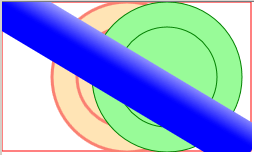
Colour gradient
The green line looks a bit boring, so I wanted to add a colour gradient, making it look 3-dimensional. All the examples I’ve seen are of horizontal or vertical boxes, but I needed the shading to be aligned along the axis of the diagonal line, so it looks like a round bar. My intention was to create some very clever code to do this, but the result always looked terrible, so in the end I just hacked the parameters to make it look roughly right. Sorry!
lg = svgwrite.gradients.LinearGradient(
     start=(0,0), end=(40,0),
     id="blue_grad", gradientUnits="userSpaceOnUse",
     gradientTransform="rotate(120)")
lg.add_colors(['blue','white'])
dwg.defs.add(lg)
dwg.add(dwg.line(
    (0,0), (WIDTH-1,HEIGHT-1),
    stroke="url(#blue_grad)",
    stroke_width=50))
dwg.save()
Modifying objects
In the above code, we’ve been creating a graphic object and and adding it to the drawing in a single line. Alternatively, we can access and modify the object’s attributes using its dictionary, for example changing the stroke colour:
line = dwg.line((10,0), (110, 100), stroke="red")
...
# Change to green using either..
line["stroke"] = "green"
# ..or..
line.update({"stroke":"green"})
...
dwg.add(line)
Javascript
The intention is to create a working seven-segment clock display; we could possibly do this in Python by continually updating an SVG file, and persuading the browser to reload it, but a much simpler method is to use Javascript.
Each object (or group of objects) to be animated must have a unique ‘id’ tag.
dwg.add(dwg.line((20,0), (120, 100), stroke="red", id="myline"))
To change this line, we have to wait until the browser has loaded the graphics, so the code is triggered by window.onload event:
SCRIPT = """
window.onload = function()
{
    var myline = document.getElementById("myline");
    if (myline)
        myline.setAttribute("stroke", "yellow");
}
"""
dwg.defs.add(dwg.script(content=SCRIPT))
That’s how easy it is to modify a graphic at run-time using Javascript.
If you are a newcomer to that language, the developer’s console in the browser is incredibly useful; you can add diagnostic printouts using console.log(), and they will only show up when the developer tools are enabled. Here is the Chrome console when ‘console.log(myline);’ has been added to Javascript; hovering the cursor over the text display causes the associated graphic bounding box to be highlighted:

SVG clock
I started off by drawing the segments using simple flat-colour lines:

However the colour gradients look much more attractive..
..so I decided to use them instead. This triggered a cascade of problems, because using colour gradients on lines is much more restrictive than rectangles, in respect of the overall dimensions the browser uses to calculate gradient values (see the documentation on gradientUnits); when lines are drawn in various on-screen positions using the same gradient, only one is the correct colour.
The way round this problem was to draw only one shaded line, then use the ‘transform’ function to rotate and move a copy of that line. The parameters for the transformation are in the form of a 6-value array, which allows complex changes to be made in one step. Simplistically, the following transformations can be made:
(1, 0, 0, 1, x, y)          Move (translate) by x,y
(sx, 0, 0, sy, 0, 0)        Scale by sx, sy
(cos, sin, -sin, cos, 0, 0) Rotate by angle
(1, 0, tan, 1, 0, 0)        x-skew by angle
(1, tan, 0, 1, 0, 0)        y-skew by angle
A transformation array is needed for each of the 7 segments, so if segment A is the original drawn line:

..the 7 segment transformations are..
# Transform matrix for each segment
SEG_MATRIX = ((1, 0,  0, 1,      0,        0), # A
              (0, 1, -1, 0, SEGLEN,        0), # B
              (0, 1, -1, 0, SEGLEN,   SEGLEN), # C
              (1, 0,  0, 1,      0, SEGLEN*2), # D
              (0, 1, -1, 0,      0,   SEGLEN), # E
              (0, 1, -1, 0,      0,        0), # F
              (1, 0,  0, 1,      0,   SEGLEN)) # G
The resulting lines are in a rectangular grid; the final flourish is to use a ‘skew’ transformation on the complete digit to give it a lean to the right:
# Matrix to slightly skew the displays
SKEW_MATRIX = "matrix(1,0,-0.1,1,0,0)"
...
g = Group(transform=SKEW_MATRIX)
The remaining question is how to do the animation; the simplest (and hopefully fastest) method I could think of is to stack all the digits 0 – 9 on top of each other, setting them transparent (opacity = 0). Each one is labelled with its position on the display, and its value, so ‘digit00’ is the left-most digit, with a value of 0, ‘digit01’ is the left-most digit with a value of 1, ‘digit10’ is the second digit with a value of 0, and so on. All the Javascript code has to do is set the opacity on the required digits, so to display the number 2345, digit02, digit13, digit24, and digit35 are opaque, the rest are transparent.
Source code
Here is the entire source code, compatible with Python 2.7 or 3.x
To view the resulting SVG file, click here.
# SVG clock with 7-segment display

import svgwrite
from svgwrite.container import Group

# 7-seg display
SEGWID      = 5             # Width & length of a segment
SEGLEN      = 20
NDIGITS     = 6             # Number of digits
DIG_PITCH   = 35            # Pitch of digits
DIG_SCALE   = 1             # Scaling factor for main digits
FRAC_SCALE  = 0.7           # Scaling factor for fractional part
LMARGIN     = 20            # Left margin
VMARGIN     = 5             # Vertical margins

GRAD_COLOURS= 'lightblue','blue'# Gradient colours
FNAME       = "svg_clock.svg"   # Filename

DWG_SIZE    = DIG_PITCH*NDIGITS, (VMARGIN+SEGLEN)*2

# Transform matrix for each segment
SEG_MATRIX = ((1,0, 0,1,0,      0),        # A
              (0,1,-1,0,SEGLEN, 0),        # B
              (0,1,-1,0,SEGLEN, SEGLEN),   # C
              (1,0, 0,1,0,      SEGLEN*2), # D
              (0,1,-1,0,0,      SEGLEN),   # E
              (0,1,-1,0,0,      0),        # F
              (1,0, 0,1,0,      SEGLEN))   # G

# Matrix to slightly skew the displays
SKEW_MATRIX = "matrix(1,0,-0.1,1,0,0)"

# Matrix to scale a segment down to a decimal point
DP_MATRIX   = "matrix(%g,0,0,1,0,0)" % (float(SEGWID)/SEGLEN)

# Segments to be activated for digits 0 - 9
dig_segs = ("abcdef", "bc", "abdeg", "abcdg", "bcfg",
            "acdfg", "acdefg", "abc", "abcdefg", "abcdfg")

SCRIPT = """
    var ndigits=6, last;

    // Initialise
    window.onload = function()
    {
        last = 0;
        setInterval(tick_handler, 100)
    }

    // Timer tick handler
    function tick_handler()
    {
        var now = new Date();
        var t = now.getHours()*10000 + now.getMinutes()*100 +
                now.getSeconds();
        if (t != last)
            set_value(t, last);
        last = t;
    }

    // Set a value on the display
    function set_value(val, oldval)
    {
        var i;
        for (i=0; i<ndigits; i++)
        {
            set_digit(ndigits-1-i, oldval, 0);
            set_digit(ndigits-1-i, val, 1);
            val = Math.floor(val / 10);
            oldval = Math.floor(oldval / 10);
        }
    }

    // Set opacity of a single display digit
    function set_digit(dig, val, op)
    {
        var digit = document.getElementById("digit"+dig%10+val%10);
        if (digit)
            digit.setAttribute("opacity", op);
    }
"""

# Create maximised SVG drawing
def create_svg(fname, size):
    return svgwrite.Drawing(fname,
            width="100%", height="100%",
            viewBox=("0 0 %u %u" % size),
            debug=False)

# Add Javascript to drawing
def add_script(dwg, script):
    dwg.defs.add(dwg.script(content=script))

# Create linear gradient, add to drawing defs
def create_lin_grad(dwg, id, start, end, colours):
    grad = svgwrite.gradients.LinearGradient(
           start=start, end=end,
           id=id, gradientUnits="userSpaceOnUse")
    grad.add_colors(colours)
    dwg.defs.add(grad)

# Create a single segment, add to drawing defs
def create_seg(dwg, id, length, width, stroke):
    seg = dwg.line((0,0), (length,0), id=id,
                   stroke="url(#%s)" % stroke,
                   stroke_width=width, stroke_linecap="round")
    dwg.defs.add(seg)

# Create digits 0 - 9 by transforming a segment, add to drawing defs
def create_digits(dwg, digid, segid):
    for dig, segs in enumerate(dig_segs):
        g = Group(id="%s%u" % (digid,dig), transform=SKEW_MATRIX)
        for seg in segs:
            num = ord(seg) - ord('a')
            mat = SEG_MATRIX[num]
            g.add(dwg.use('#'+segid, transform="matrix%s" % str(mat)))
        dwg.defs.add(g)

# Create decimal point by scaling a segment, add to drawing defs
def create_dp(dwg, dpid, segid):
    g = Group(id=dpid, transform=SKEW_MATRIX)
    g.add(dwg.use('#'+segid, transform=DP_MATRIX))
    dwg.defs.add(g)

# Add seven-segment display
# Each digit is a group of coincident transparent chars 0 - 9
def add_display(dwg, pos, pitch):
    dpos = list(pos)
    for n in range(0, NDIGITS):
        scale = DIG_SCALE if n<4 else FRAC_SCALE
        g = Group(transform = "translate(%g %g) scale(%g)" %
            (dpos[0], dpos[1], scale))
        for i in range(0, 10):
            g.add(dwg.use("#dig%u"%i, id="digit%u%u"%(n,i), opacity=0))
        dwg.add(g)
        if n == 2:
            dwg.add(dwg.use("#dp", insert=(dpos[0]-SEGLEN*0.7,
                                           dpos[1]+SEGLEN*2)))
        dpos[0] += pitch * scale

if __name__ == '__main__':
    dwg = create_svg(FNAME, DWG_SIZE)
    add_script(dwg, SCRIPT)
    create_lin_grad(dwg, "blue_grad", (0,0), (0,SEGWID*3/4),
                    GRAD_COLOURS)
    create_seg(dwg, "seg", SEGLEN, SEGWID, "blue_grad")
    create_digits(dwg, "dig", "seg")
    create_dp(dwg, "dp", "seg")
    add_display(dwg, (LMARGIN, VMARGIN), DIG_PITCH)
    dwg.add(dwg.text("iosoft.blog",
            (LMARGIN-2+DIG_PITCH*4, DWG_SIZE[1]-5),
            style="font-size:8px; font-family:Arial", fill="gray"))
    dwg.save(pretty=True)

# EOF
Copyright (c) Jeremy P Bentham 2019. Please credit this blog if you use the information or software in it.
