To debug embedded systems, such as those with the Raspberry Pi Pico processor, normally only two options are available: using ‘print’ statements, or a debug utility such as GDB. This project offers an alternative, which isn’t as invasive as the ‘print’ method, and isn’t as complex as GDB. It basically provides an insight as to the functioning of the processor and peripherals, while they are running – the CPU need not be halted to do the measurements, and the indications are equally relevant for C or Python programs.
Sadly, I can’t promise that this utility will automatically find bugs in your code; in operation, it is more like a test meter that is used to check the voltages and currents in an electrical circuit; it will show you what is going on, and give you pointers to the hardware or software areas that might be malfunctioning.
There are major differences between the on-chip debug resources for the RP2040 and RP2350; the latter is far more complex, with the potential for using much more sophisticated debug techniques. However, at the time of writing, the RP2350 is still quite a new processor, and has not yet achieved widespread usage. So the current version of PicoReg concentrates on debug features that are common to both devices; later versions will make use of the advanced features of the RP2350 to provide more sophisticated debug capabilities.
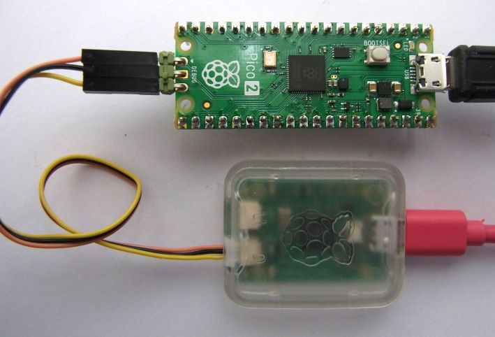
For ease of use, the PicoReg utility is written in pure Python, so it will run on a Windows or Linux PC, or a Raspberry Pi board. The interface to the target CPU is via the standard low-cost Raspberry Pi Debug Probe, with a USB interface to the PC or Pi, and a 3-wire SWD interface to the target system.
Connecting the target system
Connect the target system to the debug probe as described in the Raspberry Pi documentation, either using a 3-pin 0.1 inch pitch header as shown above, or the 3-pin miniature JST connector that is fitted to the ‘H’ variants of the Pico boards (e.g. RP2040H). It is important to keep the SWD cable short, ideally a maximum of 6 inches or 15 cm, with a good ground connection, since the signals are quite fast (10 MHz).
The Pi Debug Probe has an ARM-standard ‘CMSIS-DAP’ USB interface, and you can find other low-cost CMSIS-DAP probes online, however they probably won’t work without significant modifications to the Python code, so are not recommended.
A benefit to this setup is that it is exactly the same as used with OpenOCD, so is compatible with all the standard Pico software tools; you don’t need to re-plug the target system when switching between programming and debugging.
Installing PicoReg
The source code can be found on github here and can be copied into any convenient directory.
The files are:
picoreg.py:            main program
picoreg_disp.py:       display code
picoreg_swd.py:        SWD interface
picoreg_arm.py:        ARM CPU interface
rp2040.svd:            ARM register definitions for RP2040
rp2350.svd:            ARM register definitions for RP2350
icons/led_red_off.png: icon for I/O display
icons/led_red_on.png:  icon for I/O display
The register definition files have been taken directly from the Pico SDK, and have been provided as a convenience; they can be replaced with more up-to-date versions from the SDK, but do ensure the filenames are all in lower-case.
It is necessary to install PyQt5, pyusb, and libusb_package, e.g. for Linux:
If debug probe lacks the necessary access permission, create /etc/udev/rules.d/50-usb-cmsis.rules with the following line: SUBSYSTEM=="usb", ATTR{idVendor}=="2e8a", ATTRS{idProduct}=="000c", MODE="0666"
On newer Linux systems, the pip install method may fail with the error message “This environment is externally managed” . You can find guidance online as to the correct method of handling this error; the simplest way is to override package management by appending ‘–break-system-packages’ to the pip command.
To check the USB connection to the probe, and the SWD connection to the CPU, run
python picoreg_swd.py
The response should be:
If working OK:
Found debug probe (CMSIS-DAP)
CPU ID 0BC12477 [for RP2040, or 4C013477 for RP2350]

If target board disconnected or powered down:
Target not responding

If debug probe not connected:
Probe not found
The code can be run on any Pi Linux system, but it is recommended that a Pi4 or later be used, otherwise the user interface may be a bit sluggish.
Running PicoReg
PicoReg is run using:
python picroreg.py
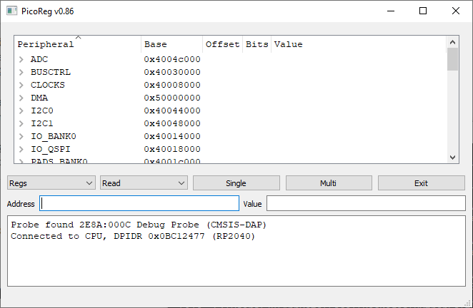
If all is well, the CPU type (RP2040 / RP2350) should be auto-detected, the appropriate SVD definition file will be parsed, and displayed in tree format.
By default, the peripheral names are sorted alphabetically; clicking on another heading will change the sorting, e.g. ‘base’ to sort by base address.
The first control (showing ‘Regs’) has a drop-down list of the various operational modes:
Regs:   Show all the CPU registers in tree format
I/O:    Display the on/off state and mode of the I/O pins
CPU:    View some of the CPU registers
Mem:    Display a block of memory or registers at a given address
PIO:    Show some of the PIO-specific registers
DMA:    Show some of the DMA-specific registers
The Regs, PIO and DMA modes are very similar, only differing in the number of registers on display. Regs mode displays the full set as defined in the SVD file, the other 2 modes show only a subset, which can make it easier to understand the operation of the selected peripheral.
The I/O display uses LED icons and text to display the state of all 29 I/O pins:
This shows the display for a typical ‘blinking LED’ program; the on-board LED on pin 25 blinks on and off, under the control of the SIO peripheral. The only other pins being controlled are pin 0 and 1, which are under the control of UART0 (asynchronous serial transmit and receive).
CPU mode shows some of the processor registers, which can be useful to check that it is running (not crashed) and give an indication of activity.
This shows that the code is running in Flash memory (10000000 hex onwards) with the stack in RAM (20000000 hex onwards).
Mem mode is used to display arbitrary areas of memory or registers (since the registers are memory-mapped).
This shows a small block of RAM that acting as a WiFi data buffer.
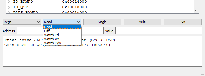
The second drop-down list selects the access mode:
Read:      Display read value
Diff:      Add the current value to a list, when the value changes
Watch Rd:  Set data watchpoint, display data on CPU write cycle
Watch Rd:  Set data watchpoint, display data on CPU read cycle
Watch R/W: Set data watchpoint, display data when CPU read or write cycle
The Read and Diff modes rely on continuous polling of the target system, at approximately 1000 times per second, so they can not capture fast changing signals. The Watch modes use the CPU hardware to detect changes, so a single rapid change will be detected, but there is a finite delay before the PC can capture the data values and re-check for another change, so multiple rapid events will not all be captured.
The ‘single’ button does one read cycle, and the ‘multi’ button runs continuous cycles until that button is pressed again.
Command-line options
Running ‘python picoreg.py -h’ produces the following help:
optional arguments: -h, --help show this help message and exit -b, --break RP2350 break on watchpoint -m MEM, --mem MEM Memory address -n NBYTES, --nbytes NBYTES Number of bytes for hex dump -r REG, --reg REG Register name -v, --verbose Enable diagnostic display -2, --core2 Use second core
The options are:
break: force the RP2350 to do a brief break on each watchpoint making its behaviour similar to the RP2040, which has to break on each watchpoint.
mem: add a specific memory address to the display. This is useful when working with a C program; the compiler generates a map file with the address of all global variables, and this option can be used (one or more times) to add addresses to the display.
nbytes: set the number of bytes to be displayed on a memory dump, the default value is 32.
reg: select a specific register to be monitored. This is case-sensitive e.g. TIMER.TIMERAWL for RP2040, or TIMER0.TIMERAWL for RP2350
verbose: display the raw CMSIS-DAP messages
2: select the second ARM core; the RP2350 RISC-V cores are not currently available
Copyright (c) Jeremy P Bentham 2025. Please credit this blog if you use the information or software in it.
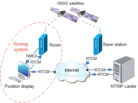
A conventional GPS (Global Positioning System) or GNSS (Global Navigation Satellite System) receiver has an accuracy that is at best 1 or 2 metres (3 or 6 feet), which is insufficient for some applications, most notably land surveys, and self-driving agricultural vehicles.
There are a few techniques that can be used to improve that accuracy, the most recent being RTK (Real Time Kinematics), which can produce centimetre-level accuracy (better than 1/2 inch). This is achieved using a receiver that can perform very detailed measurement of the satellite signal, combined with a stream of ‘correction data’ in RTCM (Radio Technical Commission for Maritime Services) format, that has been created by a nearby ‘base station’ performing continual measurements of the GNSS signal.
If you think that sounds complicated and expensive, then you’re not entirely wrong; whilst I can provide Python software that handles a lot of the complication, there is no denying that the hardware is quite expensive at present (hundreds of dollars), though there are some new devices coming on the market that could improve that situation.
GPS or GNSS
Before launching into the details, it is important to explain the difference between GPS and GNSS.
GPS is the original US group (‘constellation’) of positioning satellites, that has now been joined by systems from other countries (GLONASS, Galileo, BeiDu, NAVIC, SBAS and QZSS). The generic term for all these positioning systems is ‘GNSS’, but this term is not well known by the non-technical public, who may use the term ‘GPS’ to refer to all satellite positioning systems.
Over the years the original GPS system has evolved to cover more then one frequency band; the original L1 band at 1575 MHz has been joined by L2 at 1227.6 MHz and L5 at 1776.45 MHz. The newer bands can potentially offer better rejection of interference and handling of multipath signals, but at the time of writing, most GNSS receivers are single-band (L1 only).
Correction data
It is important that the correction data is obtained from a Base Station near the Rover; the further away the Base Station is, the worse the positioning. A theoretical figure for the accuracy is 8mm + 0.5ppm horizontal, so if the Base Station is 20 km (12.4 miles) away, the accuracy could be 18 mm (0.7 inches).
There are various ways to obtain the correction data:
Local Base Station. A Base Station can be set up nearby, with a wireless link to the Rover.
Commercial NTRIP service provider. There are commercial organisations that use NTRIP (Networked Transport of RTCM via Internet Protocol) to deliver the correction data. This can take the form of a Virtual Reference Station (VRS) that customises the data for the Rover’s location.
Free NTRIP service provider. Some free NTRIP data sources are available, but the quality and reliability may not be as good as the commercial providers.
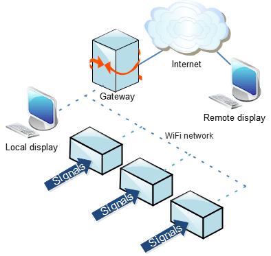
To keep the costs and complexity low, I’m using the last of these options, specifically the RTK2GO ‘caster’. This server continually takes correction signals from over 700 Base Stations world-wide; the ‘rover’ (RTK client) opens a TCP connection to the server, and requests a copy of the data from a specific Base Station. The client will then receive a continuous data stream over TCP, in the RTCM format that can be fed directly into a suitably-equipped GNSS receiver.
The advantage of this arrangement is a single Base Station can feed data to a large number of Rovers, without having to carry the burden of a lot of TCP connections; the server ‘casts’ one incoming data stream to multiple clients, and handles all the associated complexity, such as authenticating the user.
The diagram at the top of this post shows how the data flows from a Base Station to the NTRIP caster, then on to the display PC, which copies it to the GNSS receiver, which has an NMEA (National Marine Electronics Association) data output with (hopefully very accurate) position information. This must be a continuous process; if the supply of correction data stops, the GNSS receiver will drop out of RTK mode, and fall back to conventional lower-accuracy positioning.
Hardware
There are relatively few RTK-enabled GNSS receivers that can directly accept the RTCM correction data; for starters I’m using the ‘Ardusimple RTK portable Bluetooth kit’ which has the uBlox ZED-F9P receiver.
It has USB and Bluetooth interfaces that emulate a serial link, so the device appears as a COM port on a PC, and immediately starts outputting NMEA data at 115 kbaud as soon as it is powered up.
Ardusimple RTK portable Bluetooth kit
My uBlox receiver was supplied with v1.0 software, which needs to be updated using the u-center utility. If you do this without restoring the old configuration, then the receiver reverts back to 38400 baud operation; to restore this, select Configuration View, PRT (Ports) and set UART1 & UART2 to 115200 baud with NMEA enabled. One other essential configuration is to select NMEA, and tick the High Precision Mode box, to increase the number of decimal places in the position data.
When you click the ‘send’ button in the Configuration View, the settings are temporarily applied, so you can check they are correct. When the configuration view is closed, there is a prompt to save the settings to Flash, so they are non-volatile.
NMEA
NMEA (National Marine Electronics Association) have specified a standard for serial communication with GNSS devices. It takes the form of ‘sentences’, which are CRLF-terminated lines of ASCII data. The message starts with a dollar sign, the letters GP or GN, and three more letters specifying the type of sentence, then the data in comma-delimited format.
There are minor differences between different manufacturers’ implementations, so I’ve referred to the ‘u-blox F9 HPG 1.50 interface description’. It gives an example of the GGA sentence containing global positioning fix data:
The first 2 letters are the ‘talker ID’ indicating which GNSS constellation has been used, the most common are ‘GP’ indicating GPS, and ‘GN’ for any combination of satellites.
092725.00    UTC time
4717.11399   Latitude in degrees and minutes ddmm.mmmmm
N            North/south indicator
00833.91590  Longitude in degrees and minutes dddmm.mmmmm
E            East/west indicator
1            Quality 0 = No fix, 1 = GNSS fix, 4 = RTK fix, 5 = RTK float
08           Number of satellites
1.01         Horizontal accuracy (Dilution of Precision)
499.6        Altitude above mean sea level
M            Altitude units (metres)
48.0         Geoid separation
M            Geoid separation units
*5B          Checksum
The checksum is a hex value representing the exclusive-or of all the characters after the ‘$’ start, up to the checksum itself; e.g. in Python:
csum = reduce(lambda x,y: x^y, [ord(c) for c in line[1:-3]], 0)
if csum != int(line[-2:], 16):
    print("Checksum error")
A common source of confusion is that the latitude and longitude are in degrees and minutes, not decimal degrees. To perform distance calculations, they need to be converted, and combined with a North/South/East/West indication as follows:
# Convert string with degrees & minutes to decimal degrees
def degmin_deg(dm, nsew):
    deg = 0.0
    if len(dm)>=4 and nsew in "NSEW":
        n = 2 if nsew in "NS" else 3
        deg = float(dm[:n]) + float(dm[n:]) / 60.0
        deg = -deg if nsew=='S' or nsew=='W' else deg
    return deg
The serial interface uses the ‘pyserial’ project, installed using:
pip install pyserial
This package provides functions to poll the serial interface, but to ensure no characters are missed, a separate thread is used, with a Python ‘queue’ to send the completed messages to the main program:
self.rxq = Queue.Queue()

# Start thread to receive serial data
def ser_start(self):
    self.receiving = True
    self.reader = threading.Thread(target=self.ser_in, daemon=True)
    self.reader.start()

# Blocking function to receive serial data
def ser_in(self):
    line = b""
    while self.receiving:
        if self.ser.inWaiting():
            s = self.ser.read(self.ser.in_waiting)
            line += s
        n = line.find(ord('\n'))
        if n >= 0:
            self.rxq.put("".join(map(chr, line[:n+1])))
            line = line[n+1:]
        else:
            time.sleep(0.001)
The serial read function returns binary data, which is converted to a string before being added to the queue. The normal approach would be to use the ‘decode’ function to convert binary values to a string, but it is quite common for a GNSS receiver to return pure binary data alongside the NMEA sentences, and this can cause a decoding error. So the ‘map’ function is used to convert each byte to a character, which is combined into a string using the ‘join’ function.
The remaining question is how to access the individual entries within the NMEA sentence; the obvious solution is to just to index into an array of values, e.g. for GGA:
data = line[:-3].split(',')
if data[0]=='$GPGGA' or data[0]=='$GNGGA':
    fix = int(data[6])
    sats = int(data[7])
To simplify the process of naming the data fields, I tried using a ‘named tuple’ e.g.
from collections import namedtuple

# Convert string to float, return default value if failed
def str2float(str, default):
    try:
        val = float(str)
    except:
        val = default
    return val

# Define GGA sentence format
GGA = namedtuple('GGA', ['id', 'time','lat','NS','lon','EW','quality','numSV',
    'HDOP','alt','altUnit','sep','sepUnit','diffAge','diffStation'])

gga = GGA._make(data[0:len(GGA._fields)])
fix = str2float(gga.quality, 0)
sats = str2float(gga.numSV, 0)
This technique works well provided the incoming data exactly matches the sentence definition; if there is one entry to many or too few, the process fails – and it is clear from the Interface Description that there are different message lengths depending on the firmware version. So I used an alternative dictionary-based technique, that is more tolerant of message differences:
GGA_S = ('id', 'time','lat','NS','lon','EW','quality','nsats',
    'HDOP','alt','altUnit','sep','sepUnit','diffAge','diffStation')
GGA = {GGA_S[i]: i for i in range(len(GGA_S))}

# Get value from GPS sentence, given variable name
def getval(data, dict, s):
    return data[dict[s]] if dict[s]<len(data) else None

quality = str2int(getval(data, GGA, "quality"), 0)
nsats = str2int(getval(data, GGA, "nsats"), 0)
NTRIP
The satellite correction data is in RTCM (Radio Technical Commission for Maritime Services) format, sent as a continuous stream over a TCP connection using NTRIP (Networked Transport of RTCM via Internet Protocol).
As indicated above, I use the RTK2GO caster to provide the correction data, but understandably they don’t like developers using experimental clients, since it can massively increase their server’s workload. So when testing the code, it is essential to use a local host. I use SNIP for this purpose (https://www.use-snip.com/download/) running on my Windows machine, so the host is “127.0.0.1”. It is possible to run SNIP without any license payments, the only issue is that it stops working after an hour, requiring a restart. This is only a minor inconvenience, and is quite reasonable, considering the amount of functionality that it provides for free.
When running production code, the host is set to “rtk2go.com”. You can obtain a ‘caster table’ listing all the available data streams by entering http://rtk2go.com:2101 in a browser; at the time of writing there are over 700 sources.
A data connection to the server is opened using conventional TCP socket calls:
Once a connection is established, the required data must be requested; this is similar to a Web page request, with authorisation in the form of name:password that is base64-encoded. See the RTK2GO Web site for details; basically the name is an email address, and the password is usually ‘none’ unless directed otherwise.
The ‘target’ is the name of the RTCM stream; if you are using a local SNIP caster, a suitable name is ‘Demo1’.
If the request is accepted, the server will respond with the brief text message “ICY”.
RTCM
The correction data is in RTCM (Radio Technical Commission for Maritime Services) format. This protocol is designed to keep messages as short as possible, to allow them to be sent over a low-bandwidth network. So the messages aren’t text-based, they are pure binary, and the data fields aren’t necessarily aligned on byte-boundaries.
A message starts with a marker of D3 hex, followed by a 16-bit length word (M.S.byte first) then a 24-bit ‘message type’ generally with a value between 1001 and 1304 that specifies the content of that message. For example, message 1006 gives the ‘station coordinates’, i.e. the location of the data source, in an x,y,z coordinate system, known as ECEF (Earth-centred, Earth-fixed).
The data source sends each message type at a controlled rate, the maximum being 1 per second, but it can be much lower. The caster specifies the rates for each message by giving the interval between messages, e.g.
This indicates that messages 1006, 1008, 1013, and 1033 will be sent every 10 seconds, but 1074, 1084, 1094, 1114, and 1124 will be every second.
At the end of the message there is a 24-bit CRC, and the total length of each message is a maximum of 1024 bytes. Unlike some other binary serialisation protocols (such as SLIP or PPP) there is no escape code when the start marker occurs in the body of the message, so it is quite possible the message data may contain one or more D3 values. This makes the start-of-message detection somewhat complicated, since it is necessary to check the length value and the CRC to decide if the D3 is a message starter or a data byte. Additionally, each block of TCP data may contain one or more messages, or perhaps just part of a message, or just a text string, which adds to the complexity:
# Get index of byte in data, negative if not found
def bin_index(data, b):
    try:
        idx = data.index(b)
    except:
        idx = -1
    return(idx)

# Get next message from data
# If first char is not RTCM_START, then message is a text string
def get_msg(self):
    d = b""
    idx = bin_index(self.data, RTCM_START)  # Get start of RTCM block
    if idx>3 and self.data[idx-2]==0xd and self.data[idx-1]==0xa:
        d = self.data[0:idx]                # If text before RTCM..
        self.data = self.data[idx:]         # ..return text
    elif idx == 0 and len(self.data) > 2:   # Get length word
        n = (self.data[1] << 8) + self.data[2]
        if n > 1024:                        # ..check if valid
            d = self.data = b""             # Scrub data if invalid
        elif len(self.data) >= n + 6:       # If sufficient data received..
            d = self.data[0:n+6]            # ..get data
            crc = crc24(d)                  # ..check CRC
            if crc == 0:                    # If OK, remove data from store
                self.data = self.data[len(d):]
            else:
                print("CRC error")
                d = self.data = b""
    elif idx > 0:
        print("Extra data")
        self.data = self.data[idx:]
    return d
It can be worthwhile decoding the Station Coordinates (message 1005 or 1006) to establish exactly where the station is, as the Caster Table only gives the latitude and longitude to 2 decimal places. However, you can just pass the messages straight through to an RTCM-compatible GNSS receiver, without having to perform any decoding, but it is advisable to validate (CRC check) each one, to filter out unwanted SNIP text.
Sending position to Caster
The system I’ve described so far uses a unidirectional link between the Rover and the Caster; having requested the correction data, the Rover receives a constant stream of data until the connection is terminated. However there are some circumstances whereby the Caster needs to know where the Rover is, in order to provide the correct data.
Commercial casters may provide a Virtual Reference Station (VRS) which customises the correction data depending on the precise location of the Rover; RTK2GO also provides a ‘virtual’ VRS service whereby the Caster will provide the nearest data source, so ‘NEAR-England’ should provide the nearest source in England.
For these services to work, the Rover needs to send its position to the caster. The format for this message is NMEA GGA, as described above. This should not be frequent, once every 30 or 60 seconds will suffice. It is important not to retransmit every GGA message, since this is usually once per second, which risks overloading the caster with unwanted data. If the caster doesn’t need the position information (because it isn’t providing a VRS), the data will just be ignored.
Demonstration software
The demonstration software is available on Github here. It is written in v3 Python, and can run under Windows or Linux. The only library used is pyserial, installed using:
pip install pyserial
The files are:
gpsdecoder.py: serial interface to a GNSS receiver, and NMEA decode
ntripdecoder.py: NTRIP and RTCM decode
rtklient.py: console application
The console application has various command-line options, that are shown by running “python rtklient.py –help”:
usage: rtklient.py [-h] [--lat DEG] [--lon DEG] [--country STR] [-f] [-v] [-b NUM] [-c STR] [-m STR] [-p NUM] [-s URL] [-u STR]

optional arguments:
  -h, --help            show this help message and exit
  --lat DEG             latitude (decimal degrees)
  --lon DEG             longitude (decimal degrees)
  --country STR         country name (3 letters)
  -f, --find            find nearest source
  -v, --verbose         verbose mode
  -b NUM, --baud NUM    GPS com port baud rate
  -c STR, --com STR     GPS com port name
  -m STR, --mount STR   NTRIP mount point (stream name)
  -p NUM, --port NUM    NTRIP server port number
  -s URL, --server URL  NTRIP server URL
  -u STR, --user STR    NTRIP user (name:password)
This is a command-line application, so runs under the Command Prompt in Windows, or a console in Linux. Prior to running it, plug in the GNSS receiver, and note which serial port this uses; on Linux, you can see this by running ‘dmesg’, and on Windows use the Device Manager.
Run the application in a console window that is at least 90 characters wide, specifying the com port, e.g.
python rtklient.py --port com3          # For Windows
python rtklient.py --port /dev/ttyUSB0  # For Linux
If Linux refuses permission to access the port as a non-root user, a quick Internet search will explain the possible methods to correct his. If the code does not run at all, check the Python version number using “python –version”; the code requires version 3.
The program first uses the data from the GNSS receiver to establish the current position; it waits until the 3-D fix is obtained, then shows the results, e.g.
Opening port com3 at 115200 baud
Waiting for GPS position (ctrl-C to exit)..
12:33:34 51.50735112,-0.12775834,32.013 GNSS fix
Contacting NTRIP server 'rtk2go.com'
752 source table entries
Mount point not set: use --mount
To obtain correction data from RTK2GO it is necessary to specify a user name and password; this can be entered using the –user option, or by modifying the DEFAULT_USER value at the top of rtklient.py. It should contain your email address, a colon, and a password. A valid email address is essential, but for most clients, RTK2GO doesn’t actually need a password, so a value ‘none’ can be used, e.g.
DEFAULT_USER = "me@mymail.com:none"
It is also necessary to choose a ‘mount point’, i.e. a source of correction data, amongst the 752 that are currently available. The command-line option “–find” can be used to check the distance to each mount point, and print out the five nearest, e.g. for Norwich UK:
python rtklient.py --com com3 --find
Opening port com3 at 115200 baud
Waiting for GPS position (ctrl-C to exit)..
12:33:34 52.63088612,1.29735534,32.013 GNSS fix
Contacting NTRIP server 'rtk2go.com'
752 source table entries
Finding nearest mount point
  GBR             HillFarm     14.4 km
  GBR              NR152QB     14.9 km
  GBR                 IP23     39.6 km
  GBR              IP270RL     49.8 km
  GBR               JWBRTK     65.6 km
The “–mount” command-line option is used to specify the mount point, which is case-sensitive, e.g.
python rtklient.py --com com3 --mount HillFarm
Opening port com3 at 115200 baud
Waiting for GPS position (ctrl-C to exit)..
13:38:39 52.63088612,1.29735534,21.864 GNSS fix
Contacting NTRIP server 'rtk2go.com'
752 source table entries
Fetching RTCM data from HillFarm (ctrl-C to exit)
13:46:57 Pos 52.63088612,1.29735534,21.673 RTCM 1012 Dist 14253.215 RTK float
The last line is continually refreshed with a Carriage Return at the end; if the display scrolls continuously, the console window is too small, and needs to be expanded to at least 90 characters.
The RTCM value shows the latest correction message that has been received, and ‘RTK float’ indicates that the GNSS receiver is receiving the correction data, but hasn’t yet been able to get a full RTK fix; when that is achieved, ‘RTK fix’ is displayed, and the distance from the current location to the base station is shown, together with the maximum difference between the position values in metres. This gives you an idea of how much the position is changing over time, e.g.
This indicates that HillFarm is just over 14 km (nearly 9 miles) away, and with a static rover, the distance value has dithered by only 30 mm (1.2 inches).
If the receiver fails to get an RTK fix after several minutes, then the most probable cause is lack of signal from the receiving antenna; RTK does require a strong satellite signal, so it is important to have a good connection to a high-quality antenna, with a clear view of the sky.
Copyright (c) Jeremy P Bentham 2024. Please credit this blog if you use the information or software in it.
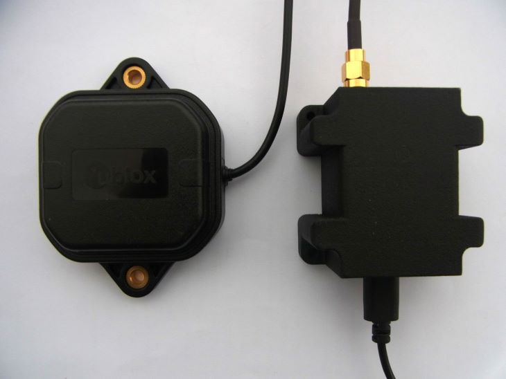
In a previous post, I described ‘EDLA’, a WiFi-based logic analyser unit, that uses a Web-based display. That version used an ESP32 to provide WiFi connectivity; the PEDLA uses a Pi PicoW module instead.
Hardware
PEDLA circuit board
The hardware is similar to the previous version; aside from the CPU change, the main addition is a 24LC256 serial EEPROM, that is used to store the non-volatile configuration parameters. The Pico flash memory can’t be used for this task, since it is bulk-erased at the start of every programming cycle. The parameters are set using a simple serial console interface.
Firmware
The firmware is written in C; networking is implemented using the picowi WiFi driver, combined with the Mongoose TCP/IP stack; follow these links for more information. The source code is on github here.
Copyright (c) Jeremy P Bentham 2024. Please credit this blog if you use the information or software in it.
Analog signal capture at 60 megasamples per second
This project provides a simple way of capturing data using a Pi PicoW, and displaying it wirelessly on a Web browser, as either as a logic analyser, or an oscilloscope.
The digital capture is done using the Pico I/O lines; the analogue capture uses an AD9226 parallel ADC module, that can provide up to 65 megasamples per second. The same firmware is used for both; for speed, the data is sent over the network as raw 16-bit values.
Hardware
In its simplest form, the only hardware required is a Pi PicoW module.
Minimal logic analyser circuit diagram
This can monitor 16 (or more) input lines, but it is essential that the voltage remains between 0 and 3.3V, otherwise damage will result. To accommodate wider voltages, an attenuator & comparator can be used, as in the EDLA project.
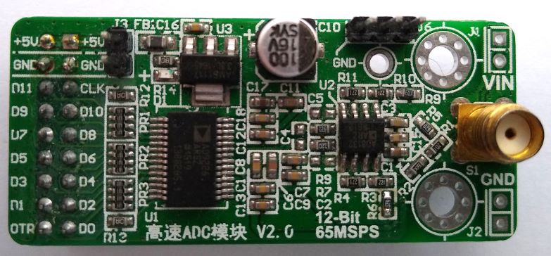
High-speed analog input uses a AD9226 ADC module, that is readily available online.
AD9226 module
It requires a 5V supply, but can be directly connected to the Pico I/O lines.
Minimal analog capture circuit diagram
Although the ADC has 12-bit resolution, only 10 bits have been used. It is possible to use all 12 bits, with minor changes to the software.
Note that some AD9226 modules have the most-significant pin marked as D0, not D11; if in doubt refer to the device datasheet, and do a continuity check between the IC pins and the I/O connections.
The ADC clock pin is connected to two I/O lines; the clock is generated on GPIO22, and read back on GPIO17. The latter is used to track the number of pulses emitted, using the pulse-counter function of the Rp2040 PWM peripheral. Any other available GPIO pins could be used instead, except that the pulse-counter function only works on odd pin numbers, so if GPIO17 is changed, it must be to an odd pin number.
When running the ADC at high speed, it is essential to keep the wiring to the Pico short (maximum 2 inches, or 5 cm) with good-quality supply & ground connections.
The analog input to the ADC module is probably 50 ohms, so can not be used with conventional oscilloscope probes. To avoid excessive loading of the input signal source, a buffer amplifier may be required.
There is a serial console output using UART1 at 115 Kbaud on GPIO pins 20 (transmit) and 21 (receive). This can be changed to use the USB link instead, by modifying the settings at the bottom of CMakeLists.txt.
Firmware
The Pico firmware is written in C; networking is implemented using the picowi WiFi driver, combined with the Mongoose TCP/IP stack; follow these links for more information. The source code is on github here.
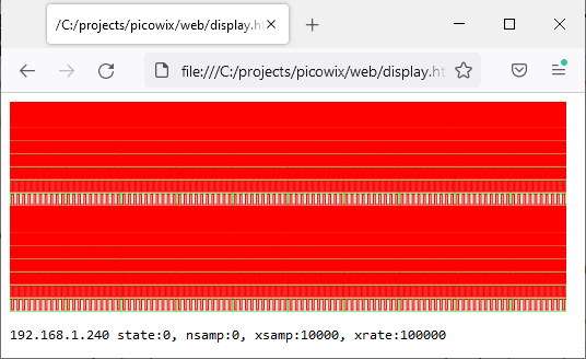
An HTTP request is used to set the parameters and initiate a capture, e.g.
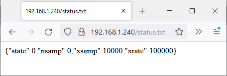
GET /status.txt?xsamp=1000&xrate=100000&cmd=1
This selects a sample count of 1000 and sample rate of 100 kHz, and the inclusion of the ‘cmd’ parameter initiates the capture.
The response is in JSON format, confirming the current state:
This confirms that 1000 samples have been captured, and are ready for transfer; if the capture is taking a long time, it will be necessary to poll the interface using a plain “GET /status.txt”, checking the ‘nsamp’ value to see when the capture is complete. If the long capture needs to be terminated, a status request with ‘cmd=0’ can be used.
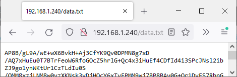
The data is fetched using:
GET /status.bin
The response is a binary block with the appropriate number of 16-bit samples. For large blocks, the transfer rate is around 2 Mbyte/s.
At the time of writing, the network details are hard-coded in the firmware, so the file ‘mg_wifi.c’ needs to be edited, to change the default network name (SSID) and password.
It may also be necessary to change the network security setting, the options are:
I have experienced difficulties with the auto-switching between protocol versions, e.g. WPA2_WPA and WPA3_WPA2; if in doubt, just use the PSK versions of WPA, WPA2 or WPA3.
When the unit powers up, the on-board LED will flash rapidly, and the serial console will display something similar to the following:
WiCap v0.26
Using dynamic IP (DHCP)
Detected WiFi chip
Loaded firmware addr 0x0000, len 228914 bytes
Loaded NVRAM addr 0x7FCFC len 768 bytes
MAC address 28:CD:C1:00:C7:D1
Joining network testnet
WiFi wl0: Nov 24 2022 23:10:29 version 7.95.59 (32b4da3 CY) FWID 01-f48003fb
Joining network testnet
WiFi wl0: Nov 24 2022 23:10:29 version 7.95.59 (32b4da3 CY) FWID 01-f48003fb
Joined network
IP state: UP
IP state: REQ
IP state: READY, IP: 192.168.43.78, GW: 192.168.43.1
The dynamic IP address will depend on the settings of your network Access Point.
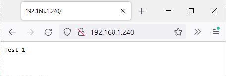
Once the unit has connected to the WiFi network, the LED will flash more slowly (1 Hz), and it should respond to network pings. A quick test is to enter the unit’s IP address in the browser’s address bar, and the unit ID and software version should be displayed, e.g. ‘WiCap v0.26’
Display software
In the ‘test’ directory there is a Javascript application to request & display the data in analog (oscilloscope) or digital (logic analyser) mode.
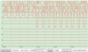
10x zoom display of 60 MS/s analog signal
Logic analyser display
The controls are:
Single / repeat: control the data acquisition, with single or multiple captures
Sample count: number of samples required (max 100,000 for RP2040)
Sample rate: frequency of capture, up to 60 MHz for a Pico with a 120 MHz clock.
IP address: the address of the capture unit. This is printed out on the unit’s serial console at power-up.
Display: retrieve data from the unit without starting a new capture cycle.
Analogue/digital: select the number of logic analyser lines to display (8 or 16) or select the analog sensitivity (0.1, 0.2, 0.5 or 1.0 volts per division).
Zoom: Select the current zoom level; the trace can be dragged left or right to the required position.
The display code is in the ‘test’ directory on github here.
Alternative client software
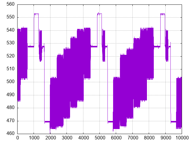
An easy way to upload the data for further processing is to use WGET, e.g.
wget http://192.168.1.2/data.bin
This returns a file containing 16-bit binary data. Then the data can, for example, be plotted using GNUPlot:
gnuplot -e "set term png; set output 'data.png'; set grid; unset key; plot 'data.bin' binary array=10000 format='%uword' with lines;"
GNUplot of analog data
Copyright (c) Jeremy P Bentham 2024. Please credit this blog if you use the information or software in it.
Mongoose TCP/IP is comprehensive easy-to-use TCP/IP software stack, produced by Cesanta Software Ltd.
In its simplest form, you just include 2 library files in your project, then can add a Web server using only 20 lines of source code, see the details here. The code is fully open-source, and the documentation is excellent; the only downside for some projects might be that a (low cost) license is required for commercial usage, but this is a reasonable request, given the amount of work that has gone into this high-quality package. Non-commercial projects can use the software for free, within the standard GPL licensing conditions.
The package supports the Pi Pico RP2040 CPU as standard, and there is an example program using the Wiznet W5500 Ethernet controller, the source code is available here. There is also an example of WiFi connectivity on the Pico-W, using the standard Raspberry Pi Application Programming Interface (API) but the result is quite complex, so I’ve replaced that API with my high-speed WiFi drivers, to produce a fast, flexible, and easy-to-use solution for TCP/IP on the Pico-W.
Mongoose
An unusual feature of the Mongoose TCP/IP software stack is that it isn’t tied to any operating system (OS); not only can run under Windows, Linux or a Real Time Operating System (RTOS), but it can also work completely standalone, with no OS at all. This is achieved by eliminating all the usual tasks, threads, semaphores, mutexes etc., and running everything within a main polling loop. This makes the code uniquely portable, and it works work well with my Picowi WiFi drivers, since they are also based on a polling methodology.
If there is no OS, how can Mongoose handle the request for Web server files, since the file-system doesn’t exist? The answer is that ‘static’ files (i.e. files that don’t change) can be embedded into the source code, and they will be returned as if they came from a conventional OS. Dynamic files can be returned by intercepting the file request, and creating a response on-the-fly.
In its simplest form, all the Mongoose source-code is in a single file, mongoose.c, with a single header file, mongoose.h, making integration into an existing code-base really easy; it is just necessary to call the polling function as often as possible, and handle the (optional) callbacks when a request is received by the Web server.
MG PicoWi
The starting-point for my project is the tutorial for Pico Ethernet using the W5500 chip, but there are some important differences between Ethernet and Wifi connectivity:
Link failures. It is highly unusual for an Ethernet link to fail, since it uses a relatively secure plug-and-socket connection. Wireless links are much less secure, since they are competing for use of a shared medium (a specific radio channel) which can become very congested, leading to a high failure rate.
Security. Since the communications medium is open to all, it is necessary to establish a secure link, as a precaution against eavesdroppers. There are various schemes in use; at the time of writing, the most common is Wi-Fi Protected Access 2 (WPA2), with WPA3 just starting to become available.
Negotiation. As a result of the above, there is a significant amount of negotiation between the unit (known as a ‘station’ or STA) and a central hub (known as an Access Point or AP) when a unit wishes to join a WiFi network, and there is the distinct possibility of failure, e.g. if the STA has the wrong WPA encryption key. Compare this with Ethernet, where is it just a question as to whether the cable is plugged in to both units or not i.e. the network is ‘up’ or ‘down’.
The above points just refer to the establishment of a Wifi link between STA and AP, but there may be other negotiations as well, most notably obtaining an Internet Protocol (IP) address using Dynamic Host Configuration Protocol (DHCP). So it is important to have a robust mechanism for handling low-level network faults, and a way of informing higher-level code that the low-level link is broken, so nothing can be sent or received. I’ve also indicated a visual indication of the connection status, flashing the on-board LED at a fast rate if disconnected, slowly if connected.
Initialising the WiFi interface
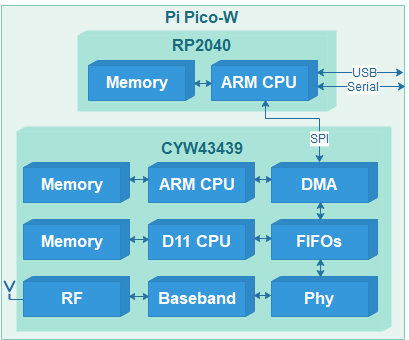
The WiFi chip on the Pi Pico W is the CYW43439, and it contains 2 CPUs, with the attendant memory and peripherals. As a result, initialising the chip is quite complex; for example, it is necessary to load 230 KB of firmware into its memory every time it is powered up. My Picowi project describes the chip initialisation in considerable detail; if you want to learn about the low-level hardware & software interfaces, see part 1 and part 2 of that project.
Once the firmware has been loaded, and the chip CPUs are running, then there are many more commands to configure the interface; these are also sent by the PicoWi software. In the event of an error, there isn’t any corrective action that can be taken, apart from power-cycling the chip, and repeating the whole initialisation process.
Joining a network
The software connects to a WiFi network, that is specified by:
SSID. This is the Service Set Identifier, a string broadcast by the Access Point (AP) containing the network name. This is not to be confused with the Basic Service Set Identifier (BSSID); this is the low-level Media Access and Control (MAC) address of the AP, which is not needed.
Encryption protocol. This specifies the method that will be used to secure the WiFi transmissions. If the network is ‘open’, then there is no security, and the transmissions can easily be monitored and intercepted. The early security protocols such as WEP (Wired Equivalent Privacy) provide minimal protection, so the more modern WPA (Wi-Fi Protected Access) is generally used, with its successors WPA2 and WPA3.
Password. This is the secret encryption key used to encode & decode the transmissions; for WPA it is a string with a length from 8 to 64 characters.
It is not unusual for the network connection attempt to fail, so the code is contained within a loop, and a retry is performed after a suitable delay.
Transmission and reception.
The Mongoose stack is designed to handle a variety of network drivers, that are specified using a single structure with pointers to functions for initialisation, transmission, reception, and network state reporting:
The transmit & receive functions call the corresponding functions within PicoWi:
// Transmit WiFi data
static size_t mg_wifi_tx(const void *buf, size_t buflen, struct mg_tcpip_if *ifp)
{
    size_t n = event_net_tx((void *)buf, buflen);
    return  n ? buflen : 0;
}
// Receive WiFi data
static size_t mg_wifi_rx(void *buf, size_t buflen, struct mg_tcpip_if *ifp)
{
    int n = wifi_poll(buf, buflen);
    return n;
}
It is important to realise that the polling of the WiFi chip isn’t just to receive data, it is also to receive other ‘events’, such as notifications of the network state. Furthermore, Mongoose does not call this function if the network is ‘down’, so there is a risk that the network will be permanently stuck in the ‘down’ state, since the WiFi chip isn’t being polled for events to show the network is ‘up’.
The solution to this problem is to include additional polling in the main loop:
if (!mif.driver->up(0))
    wifi_poll(0, 0);
This polls the WiFi interface if it isn’t reported as ‘up’, so that the change-of-state can be detected. The zero parameters ensure that in the ‘down’ state, any incoming network data is discarded, since nothing useful can arrive until the the network has been joined.
Polling
To those unfamiliar with embedded systems, the extensive use of polling might seem to be counter-productive, resulting in a much slower response to network events – wouldn’t it be quicker to use interrupts?
The answer to this question comes from a deeper understanding of what actually happens within a multi-tasking system. To give an interrupt-driven system a quick response-time, it is important that the interrupt hander doesn’t do much; it has to rapidly save the incoming data, without doing much processing, in order to be ready for the next message. So it will set a semaphore, that will wake up another process that decodes the message format and prepares a response, which is put in a queue for transmission. Then another context-switch will pass control to a transmit routine, to send the response out. It is important to ensure that the hardware isn’t being accessed by 2 routines at the same time, so mutual exclusion (‘mutex’) flags have to be used to guarantee this.
This logic is quite complex, and due to its dynamic nature, is difficult to test & debug; an error can cause the network driver to stall, until an idle-timer expires, and triggers code that tries to resolve the situation.
For this reason, the overall simplicity of single-threaded polled code can appear quite attractive; interrupts can still be used for real-time processing (such as scanning a keypad) whilst the network code keeps running in the background.
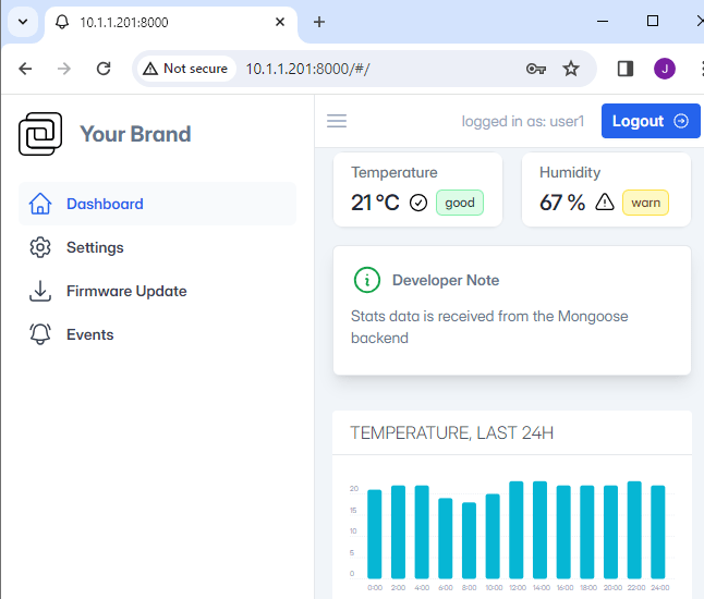
Web server
The Web server (web_server.c) is described in considerable detail in the Mongoose documentation, so there is little I can add. If you log in using one of the given identities, there is a demonstration of various features, but sadly the most interesting (such as Firmware Update) are just dummy functions; extra code is needed to make these operational.
Bulk data transfer
I have previously said that the Web server can provide static (read-only) files from its compiled-in filesystem, and small dynamic files by intercepting the file request callback, and generating the HTML code on-the fly. However there is another use-case; what happens if we want to return a very large file on-the-fly, for example, a picture from a Web camera? Cesanta have provided a ‘huge response’ example, but it involves chopping up the data into smaller sections, and reassembling them on the client using Javascript. I’d like to display the image by simply pointing the browser at its location, so this technique isn’t suitable.
There is an alternative method; just emulate a filesystem containing the file we want to send. When accessing the file, Mongoose starts by issuing a ‘stat’ call to get the data length & timestamp, then follows with an ‘open’ call, multiple ‘read’ calls, and a ‘close’ call. It is easy to intercept these file calls, since they are function pointers in a file API structure:
This is a port of the mongoose Web server and device dashboard onto the Pi PicoW, using the picowi WiFi driver in place of the conventional lwIP code.
The network details are hard-coded in the firmware, so the file ‘mg_wifi.c’ needs to be edited, to change the default network name (SSID) and password.
It may also be necessary to change the network security setting, the options are:
I have had difficulties with the WPA2_WPA and WPA3_WPA2 settings, so have generally found it best to use PSK with WPA, WPA2 or WPA3.
There is a serial console, with transmit data on pin 1 of the PicoW module, at 115200 baud. When the unit powers up, the on-board LED will flash rapidly, and the console will display something similar to the following:
WiCap v0.26
Using dynamic IP (DHCP)
Detected WiFi chip
Loaded firmware addr 0x0000, len 228914 bytes
Loaded NVRAM addr 0x7FCFC len 768 bytes
MAC address 28:CD:C1:00:C7:D1
Joining network testnet
WiFi wl0: Nov 24 2022 23:10:29 version 7.95.59 (32b4da3 CY) FWID 01-f48003fb
Joined network
IP state: UP
IP state: REQ
IP state: READY, IP: 10.1.1.78, GW: 10.1.1.1
The dynamic IP address will depend on the settings of your network Access Point.
Once the unit has connected to the WiFi network, the LED will flash more slowly (1 Hz); it should respond to network pings, and the Web server will be available on the usual port 80.
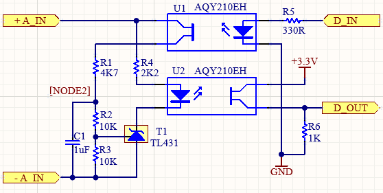
Circuit diagram of Simple Isolated Analog-to-Digital converter
This project was prompted by the need for a circuit to provide a galvanically-isolated measurement of battery voltage. Existing designs tend to be complicated, expensive or both, so a new approach was adopted, that keeps the circuitry simple, and relies on the timing capability of a CPU. I’m using a Pi Pico RP2040, but almost any microcontroller would do, so long as it has a simple pulse-timing capability.
Why does the measurement have to be isolated? In my case, the equipment is in an environment with a lot of electrical noise, so good isolation is essential, but the technique has other advantages:
Measurement of voltages that are floating with respect to ground
Avoidance of any ground-loops
Protection against transients on the lines being measured
Simple hardware that can be implemented using surface-mount or robust through-hole devices
Low-cost readily-available parts
Negligible load-current when not measuring
The last point is quite important since in battery-powered systems, we don’t want the monitoring system to act as a continuous drain on the battery itself.
Operating method
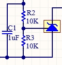
Charge / discharge of 1 uF capacitor with 1K resistor and 10V supply
A standard method for converting an analogue voltage to digital is the dual-slope ADC, whereby the time taken to charge a capacitor to the unknown voltage is compared with the time taken for a known ‘reference’ voltage; the ratio of the two indicates the value of the unknown voltage.
One obvious simplification would be to just use a single slope; measure the time taken to charge the capacitor to a known voltage, and since capacitor-charging follows a known exponential curve, a simple equation would yield the voltage value.
The big problem with this approach is the capacitor itself; there are many types of capacitor, but they all share the same characteristic to a greater-or-lesser extent: their capacitance value is not very accurately defined. If you look through a typical electronics catalogue, there aren’t many capacitors below 10% tolerance, and many are far worse than that. Then there is the issue of the capacitor value changing with temperature & age, and even in some cases, the applied voltage.
So it is important to minimise the effect of a change in capacitance, by basically comparing the time taken to charge up using the unknown voltage with the time taken to discharge from a known voltage. The charge & discharge times can easily be measured by a microcontroller, using digital signals that have been passed through an opto-coupler to provide isolation.
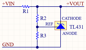
Shunt voltage reference
The TL431 is known as a ‘shunt voltage reference’ since its primary function is to clamp a voltage to a known value. It is also known as a ‘programmable zener diode’ which accounts for the surprising terminology, whereby the anode is the negative terminal, and the cathode is the positive terminal. The anode-cathode junction is essentially open-circuit until the voltage of the reference pin is around 2.5 volts (2.470 to 2.520 V according to the TL432A datasheet), when that junction will conduct. So in the above circuit diagram, if R2 and R3 are equal, and the input voltage is over 5V, then the output voltage will be clamped to 5 volts.
However the cathode line doesn’t necessarily have to go to the R1 R2 junction; in my design it goes to an optocoupler diode. This means that the opto will be energised when the gate pin reaches 2.5 volts. An additional side effect (not explicitly mentioned in the datasheet) is that the gate line is clamped to 2.5V; this becomes relevant when simulating the circuit.
Charge cycle
To satisfy the requirement for near-zero current when not measuring, a digital signal (through an opto-coupler) is used to start the measurement. I’ve used a FET opto-coupler, since its close-to-zero on-resistance is useful for simplifying the design, but a conventional Bipolar Junction Transistor (BJT) type could be used instead, taking into account the voltage drop across its emitter-collector junction.
Capacitor C1 is charged through R1, with resistors R2 & R3 acting as a load across the capacitor. Once the capacitor is fully charged, the voltage across it will be:
VCmax = VIN * (R2+R3) / (R1+R2+R3)
So if the input is 12V, the final voltage across C1 will be 9.717 volts. The standard value for measuring the charge-time of a capacitor is the ‘time constant’, which is the time taken to charge it to 63.2% of the final voltage, and if R2 and R3 weren’t there, this would be equal to C1 * R1, which is 4.7 milliseconds. The effect of C2 and C3 is to reduce the time-constant as if R2 + R3 were placed in parallel with R1, so the time-constant becomes:
TC = C1 * (R1 * (R2 + R3) / (R1 + (R2 + R3)))
This reduces the time-constant to 3.806 ms. The equation for the voltage across C1 is:
V = VS * (1 - exp(-T / TC))
Where:
    VS is supply voltage
    T is time in seconds
    TC is time-constant (C * R)
It follows that the equation to calculate the time to reach a given voltage is:
T = -log(1 - (V / VS)) * TC
The way we’ll measure charge-time is start a clock when the opto-coupler is energised, and stop that clock when the TL431 device switches on; since R2 has the same value as R3, the switch-on will happen when the voltage across C1 is 5V. So the time to switch on for a 12V supply will be:
-log(1 - (5 / VCmax)) * TC = 0.002751 seconds
Discharge cycle
Once the voltage across C1 has stabilised, the CPU can switch off the supply to the U1 optocoupler, and the voltage across C1 will decay; when it falls below 5V, the TL431 will switch off, switching off U2. So the discharge time is measured between U1 and U2 being switched off.
Charge / discharge simulation for 10V supply
The discharge time would be quite easy to calculate were it not for the fact that the TL431 clamps the reference pin to 2.5 volts with respect to the anode, so the discharge isn’t a simple exponential curve.
The best way to calibrate the ADC is to use known supply voltages, and use the microcontroller to report the charge & discharge times, and the ratio between them, e.g.
The tests have been done in descending order, so the time ratios are in ascending order, which simplifies the process of converting a measured time ratio into a voltage using linear interpolation:
There is plenty of scope for changes or improvements to this design; for example, the current component values give a useful measurement range of 8 to 20 volts, which can be increased by changing R1, though it is necessary to bear in mind the ‘absolute maximum’ anode-cathode voltage of the TL431, which is 37 volts.
The capacitor value can be increased to give longer charge & discharge times, but the overall measurement time will increase as well, as the discharge cycle should only be started when the capacitor is fully charged. A suitable candidate would be a 10 uF tantalum device, but don’t use a wide-tolerance part such as an aluminium electrolytic, if you want the measurements to have long-term repeatability.
Copyright (c) Jeremy P Bentham 2023. Please credit this blog if you use the information or software in it.
In a previous post, I looked at ways of measuring frequency accurately using an RP2040 CPU programmed in C. In this project, I have re-coded those functions in MicroPython, and provided a few enhancements.
I use Direct Memory Access (DMA) to minimise the CPU workload, and avoid the need for interrupts, but this raises a problem: when programming in C, there is a substantial Application Programming Interface (API) that allows everything on the RP2040/2350 chip to be configured using simple function calls. However, MicroPython aims to be more-or-less compatible with a wide range of CPUs, so not much CPU-specific code has been included. This means that we have to do some low-level programming if we want to use the more obscure functions of the Pulse Width Modulation (PWM) peripheral.
My first attempt at ADC and DMA low-level programming used MicroPython ‘uctypes’ to create a model of the peripherals, and if you are interested in the nuts-and-bolts of this method, I suggest you browse the post here.
This approach produced excellent results, but wasn’t very ‘pythonic’, so I’ve encapsulated common API functions in Python classes; when choosing function names, I’ve copied those in the C API when possible. So for example, setting the PWM peripheral in C is:
In MicroPython this is done by instantiating a device from the PWM class:
import pico_devices as devs
PWM_GPIO_PIN = 3
pwm = devs.PWM(PWM_GPIO_PIN)
pwm.set_clkdiv_mode(devs.PWM_DIV_B_RISING)
# ..and any other settings..
Not only are the function call names very similar between C and Python, but also the underlying code is similar; for example, the set_clkdiv function is defined as:
class PWM:
    def set_clkdiv_mode(self, mode):
        self.slice.CSR.DIVMODE = mode
where ‘slice’ is the (somewhat unusual) name for a PWM channel, CSR is the Control and Status Register, and DIVMODE is a 2-bit field within that register. If you want to learn more about the internal structure of the PWM peripheral, I suggest you take a look at the C language post.
The Python classes have been kept very ‘lean’, with no error-checking of the parameters; when time permits, I intend to create a sub-class that provides comprehensive parameter-checking .
The initial version of the post was RP2040-only; for the RP2350 CPU on the Pico2 the underlying logic is the same, but a few details had to be changed, as detailed towards the end of this post.
Test signal
We need a waveform for the tests, which the RP2040 PWM peripherals can easily provide. The following code generates a 100 kHz square wave on GPIO pin 4:
The choice of GPIO pin number is quite arbitrary, you just need to be aware when programming PWM that there are are 16 channels (technically 8 slices, each with 2 channels) mapped onto 32 pins, so if I’m using GPIO pin 4 for this signal, I can’t use PWM on GPIO 20. However, that pin is still available for any other purpose, so the limitation usually isn’t a problem.
16-bit counter
The RP2040 PWM peripheral can also act as a pulse counter, and by counting the number of edges in a given time, we can establish the frequency. This pulse input capability is only available on odd GPIO pin numbers (i.e. channel B of a PWM ‘slice’).
The code is quite simple; it is only necessary to set the mode, and the frequency divisor:
# Initialise PWM as a pulse counter (gpio must be odd number)
def pulse_counter_init(pin, rising=True):
    devs.gpio_set_function(pin, devs.GPIO_FUNC_PWM)
    ctr = devs.PWM(pin)
    ctr.set_clkdiv_mode(devs.PWM_DIV_B_RISING if rising else devs.PWM_DIV_B_FALLING)
    ctr.set_clkdiv(1)
    return ctr
Now we can make a simple frequency meter, by clearing the count to zero, then enabling the counter for a specific period of time:
# Enable or disable pulse counter
def pulse_counter_enable(ctr, en):
    if en:
        ctr.set_ctr(0)
    ctr.set_enabled(en)

# Get value of pulse counter
def pulse_counter_value(ctr):
    return ctr.get_counter()

pulse_counter_enable(counter, True)
time.sleep(0.1)
pulse_counter_enable(counter, False)
val = pulse_counter_value(counter)
print("Sleep 0.1s, count %u" % val)
The count-value for a 100 kHz signal and a 100 millisecond sleep is theoretically 10000, but is actually around 10015, due to the time-delays associated with the Python instructions. I’ll be describing ways to eliminate these delays later on in this post.
32-bit counter
Unfortunately the PWM peripheral has only a 16-bit counter, which can be too short for high-frequency signals or long sample-times. In the C code I polled the count value, to count the number of times it rolled over past 65535, then add on that number to the final result.
An alternative method is to take advantage of the fact that the DMA controller has a 32-bit down-counter that decrements every time a DMA cycle is completed. So we just need to set the DMA count to a large number, and set the PWM peripheral to trigger a DMA cycle on every rising or falling edge of the input signal.
This prompts the question “what data should the DMA transfer?” and the answer is “anything: it doesn’t matter”, but we still have to be careful to ensure the transfers don’t over-write some random area in memory. We need to very carefully specify the DMA source & destination addresses, using the binary ‘array’ data type, which occupies a fixed area of memory, without all the complexities of a Python ‘object’. The syntax to create the array is somewhat unusual; rather than just specifying a size, we have to provide the initial data using an iterator. The pico_devices library provides a helper function to simplify the process:
# Create 32-bit array (to receive DMA data)
def array32(size):
    return array.array('I', (0 for _ in range(size)))
To use this array with DMA, we have to get its address in memory, using ‘uctypes.addressof’:
# Get address of variable (for DMA)
def addressof(var):
    return uctypes.addressof(var)
Armed with these functions, we can initialise the DMA controller:
ext_data = devs.array32(1)  # Dummy array for extended counter

# Use DMA to extend pulse counter to 32 bits
def pulse_counter_ext_init(ctr):
    ctr.set_enabled(False)
    ctr.set_wrap(0)
    ctr.set_ctr(0)
    ctr_dma = devs.DMA()
    ctr_dma.set_transfer_data_size(devs.DMA_SIZE_8)
    ctr_dma.set_read_increment(False)
    ctr_dma.set_write_increment(False)
    ctr_dma.set_read_addr(devs.addressof(ext_data))
    ctr_dma.set_write_addr(devs.addressof(ext_data))
    ctr_dma.set_dreq(ctr.get_dreq())
    ctr.set_enabled(True)
    return ctr_dma
We’re modifying the PWM 16-bit counter to wrap around to zero on every input edge, and initialising its starting value to zero, which is essential. Then a DMA channel is instantiated, and configured to copy 8 bits from the data array back to the data array.
It is important to note that enabling the DMA counter does not necessarily start the transfer from scratch; if a transfer has already started, the controller will resume counting where it left off. So it is necessary to clear out any existing transfer, before stating a new one:
# Start the extended pulse counter
def pulse_counter_ext_start(ctr_dma):
    ctr_dma.abort()
    ctr_dma.set_trans_count(0xffffffff, True)

# Stop the extended pulse counter
def pulse_counter_ext_stop(ctr_dma):
    ctr_dma.set_enable(False)

# Return value from extended pulse counter
def pulse_counter_ext_value(ctr_dma):
    return 0xffffffff - ctr_dma.get_trans_count()
Using the extended pulse counter is similar to the 16-bit counter, we just need to remember the limitation that if the 32-bit value is exceeded, the counter will stop, and not wrap around.
This shows that the count is not limited to 16 bits.
Gating a counter
To accurately count pulses with a specific time-frame, it is necessary for the timing to be accurate, and as we have seen, the ‘sleep’ function introduces a significant error. To eliminate this, we need a hardware mechanism whereby a timer directly enables and disables the counter (a process called ‘gating’) without requiring any intervention from the CPU.
This involves programming another PWM channel to act as a timer, then when the time has expired, using DMA to modify the counter’s register to stop counting. The default PWM clock is 125 MHz, the prescaler is 8 bits, and the counter register is 16 bits, effectively 17 bits if we engage ‘phase correct’ mode. So the slowest gate frequency is 125e6 / (256 * 65536 * 2) = 3.725 Hz, a gate-time of 0.268 seconds; I’ve opted for 0.25 seconds.
This code uses GPIO pin 0 to identify which PWM ‘slice’ is being used. Since we aren’t enabling PWM I/O on that pin, it can still be used for any other function, such as serial output.
We need to trigger a DMA cycle when the gate PWM times out; that cycle will be used to disable the counter PWM. So when initialising the DMA channel, we need to capture the non-enabled state, that will be written into the counter CSR register; this is only one 32-bit value, but I’m using a fixed array for that value, since DMA can’t handle the complexities of Python object storage.
To start the frequency measurement, it is necessary to set the DMA count (since this is reset by a DMA cycle), enable DMA, then enable the gate & counter PWM devices simultaneously.
# Start frequency measurment using gate
def freq_gate_start(ctr, gate, dma):
    ctr.set_ctr(0)
    gate.set_ctr(0)
    dma.set_trans_count(1, True)
    ctr.set_enables((1<<ctr.slice_num) | (1<<gate.slice_num), True)
If all is well, the test signal frequency should be reported correctly on the console:
Gate 250.0 ms, count 25000, freq 100.0 kHz
Edge timer
An alternative method for measuring frequency is to measure the times between the rising or falling edges, producing values that are the reciprocal of the frequency. This is particularly useful when dealing with slow signals, or if you want to implement a method to eliminate ‘rogue’ pulses, since you get one measurement for each cycle of the input signal, so could reject pulses that are outside the expected frequency range.
By now, you won’t be surprised to learn that I use DMA to capture the time-value for each edge; there is a convenient 32-bit microsecond-value that can be copied into a suitably-sized array on edge positive or negative edge; the sole function of the PWM peripheral is to detect the edge, and trigger a DMA cycle.
We’ll be generating a test signal as before, but this time it is 10 Hz:
Starting the DMA is a bit different; firstly we need to use the ‘abort’ command to stop any previous transfer that might still be in progress. If we didn’t do that, and just enabled DMA, the transfer would resume where it left off – the new settings would be ignored. Secondly we need to set both the transfer count and the destination address, since these will have been changed by a previous transfer.
# Start frequency measurment using gate
def timer_start(timer, dma):
    timer.set_ctr(0)
    timer.set_enabled(True)
    dma.abort()
    dma.set_write_addr(devs.addressof(time_data))
    dma.set_trans_count(NTIMES, True)
The main program needs to perform some simple maths to derive the frequency, guarding against the possibility that there may be insufficient time-values (1 or less):
NTIMES = 9                       # Number of time samples
time_data = devs.array32(NTIMES) # Time data

timer_pwm = timer_init(PWM_IN_PIN)
timer_dma = timer_dma_init(timer_pwm)

timer_start(timer_pwm, timer_dma)
time.sleep(1.0)
timer_stop(timer_pwm)

count = NTIMES - timer_dma.get_trans_count()
data = time_data[0:count]
diffs = [data[n]-data[n-1] for n in range(1, len(data))]
total = sum(diffs)
freq = (1e6 * len(diffs) / total) if total else 0
print("%u samples, total %u us, freq %3.1f Hz" % (count, total, freq))
The frequency of the test signal should be displayed on the console:
9 samples, total 800000 us, freq 10.0 Hz
Running the code
The source files are available on Github here. It is necessary to load the library file ‘pico_devices.py’ onto the target system; if you are using the Thonny editor, this is done by right-clicking the filename, and selecting ‘Upload to /’. You can then run one of the program files to measure frequency:
pico_counter.py: use simple pulse counting and sleep timing
pico_freq.py: use DMA to accurately gate the pulse counter
pico_timer.py: use time-interval (reciprocal) measurement
Don’t forget to link GPIO pin 4 (the test signal output) to pin 3 (the measurement input) for these tests.
Pico2 RP2350 processor
Some minor changes had to be made to accommodate the newer processor; for simplicity, the code in pico_devices.py auto-detects which platform it is running on, and alters the settings accordingly.
Identifying the CPU
There is a Micropython library function uos.uname() that provides CPU identification. Here is the output, running on the latest Micropython versions at the time of writing (the full Pico2 release isn’t available yet):
# Response on RP2040 Pico
(sysname='rp2', nodename='rp2', release='1.23.0', version='v1.23.0 on 2024-06-02 (GNU 13.2.0 MinSizeRel)', machine='Raspberry Pi Pico with RP2040')

# Response on RP2350 Pico2
(sysname='rp2', nodename='rp2', release='1.24.0-preview', version='v1.24.0-preview.321.g0ff782975 on 2024-09-23 (GNU 14.1.0 MinSizeRel)', machine='Raspberry Pi Pico2 with RP2350')
Since the code should be compatible with any board that uses an RP2350, I decided to set a boolean variable by checking the ‘machine’ string for the number ‘2350’, e.g.
PICO2 = "2350" in uos.uname().machine
Clock frequency
The default clock frequency for the Pico2 is 150 MHz, as opposed to 125 MHz for the RP2040. This increase highlights an unfortunate problem with the divisor values I’ve previously chosen; to get a 250 ms gate-time, I prescaled the clock frequency by 250 to get 500 kHz, then divided by 125000 to get 4 Hz. However, this doesn’t work with the higher clock frequency, since the prescaler is restricted to an 8-bit value, and the divisor to a 17-bit value (since I’m using ‘phase correct’ mode); the lowest frequency I can get on the Pico2 is 4.49 Hz, so I’m using 5 Hz:
Although the structure of the CPU peripherals remains unchanged, there are various changes to the details. The most obvious of these are the base addresses:
Refer to pico_devices.py to see all the changes, but in practice the differences can be ignored, as the values change automatically, based on identification of the CPU.
Copyright (c) Jeremy P Bentham 2024. Please credit this blog if you use the information or software in it.
This project describes the creation of the software for a vehicle speedometer. It measures the frequency of a signal that is proportional to speed, but I’m also using the opportunity to explore two possible techniques for measuring frequency with high accuracy using an RP2040 processor.
Unusually, I’m going to use the RP2040 PWM (Pulse Width Modulation) peripheral to count the clock pulses. PWM is normally used to generate signals, not measure them, but the RP2040 peripheral has an unusual feature; it can be use to count pulse-edges, namely the number of low-to-high or high-to-low transitions of an input signal. If we start this counter, and stop after a specific time (which is commonly known as ‘gating’ the counter) then we obtain the frequency by dividing the count by the time.
The RP2040 documentation uses the unusual term ‘slice’ to denote one of the PWM channels, where each slice has 2 ‘channels’ (A and B) that are associated with specific I/O pins, as follows:
Slice 0 channel A uses GPIO 0, Slice 0 channel B uses GPIO 1
Slice 1 channel A uses GPIO 2, Slice 1 channel B uses GPIO 3
Slice 2 channel A uses GPIO 4, Slice 2 channel B uses GPIO 5
..and so on..
When generating PWM signals both channels can be used, but when counting edges we must use the ‘B’ channels, so an odd GPIO pin number.
The PWM counter isn’t difficult to set up, using the standard Pico hardware interface library:
The sleep_msec() call isn’t very accurate, its timing will depend on other activities the RP2040 is performing (such as USB interrupts).
During the sleep_ms() call the CPU is just wasting time, doing nothing; if we want to do something else (such as scanning a button input) then we’ll have to use a timer interrupt for that, which will further reduce the accuracy of the sleep timing.
The count is a 16-bit number, so we must choose a gate-time that ensures the counter won’t overflow.
To fix points 1 & 2 we need the gating timer to be implemented in hardware, and we can use another PWM ‘slice’ for this purpose; it is basically acting as an up-counter fed from a known clock, and when it times out, we halt the counter PWM, so its value is fixed.
To achieve good accuracy, there should also be a hardware link between the timeout of the timer PWM and the stopping of the counter PWM, so it won’t matter what code the CPU is executing at the time. Fortunately the timer PWM can trigger a DMA (Direct Memory Access) cycle when it times out, and we can use this cycle to update the counter PWM control register, stopping the counter. This means that once the two PWM slices are started (counter & timer) no more CPU intervention is required, until the data capture is finished.
Initialising the gate time & DMA is a little more complicated:
The PWM wrap settings deserve some explanation; since the hardware register is 16 bits, the obvious choice is to set the timer wrap value to 65536 or less, but this means the longest gate-time is 65536 * 256 / 125 MHz = 134 msec. However, by selecting ‘phase correct’ mode, the PWM device counts up to the wrap value, then back down again, before triggering the DMA. So the wrap value effectively becomes 17 bits wide, and we can set a gate time of 250 msec, as in the code above.
To run a capture cycle, it is only necessary to give the DMA controller the address of the register to be modified (the counter PWM ‘csr’ register) and start both PWM slices simultaneously.
To get read the counter value, we need to wait until the DMA cycle is complete, then stop the timer and access the count register.
// Get pulse count
int counter_value(void)
{
    while (dma_channel_is_busy(gate_dma_chan)) ;
    pwm_set_enabled(gate_slice, false);
    return((uint16_t)pwm_get_counter(counter_slice));
}
There is still the problem of the counter potentially overflowing if there is a high-frequency input; this could be solved using a PWM overflow interrupt, but personally I prefer to poll the count value to check for overflow, for example:
uint counter_lastval, counter_overflow;

// Check for overflow, and check if capture complete
bool counter_value_ready(void)
{
    uint n = pwm_get_counter(counter_slice);

    if (n < counter_lastval)
        counter_overflow++;
    counter_lastval = n;
    return (!dma_channel_is_busy(timer_dma_chan));
}
A capture cycle that is protected against counter overflow could now look like:
counter_start();
while (!counter_value_ready())
{
    // Insert code here to be executed while waiting for value
}
printf("%u Hz\n", frequency_value());
Reciprocal measurement
The ‘count-the-edges’ technique described above works well for reasonably fast signals (e.g. 1 kHz and above), but at lower frequencies it is quite inaccurate, so an alternative technique is used, which is known as ‘time-interval’ or ‘reciprocal’ measurement.
Instead of counting the number of transitions in a given time, the new technique measures the time between the transitions, for one or more cycles; the inverse of this time is the frequency.
We have already seen how the RP2040 PWM peripheral can be used to count pulses and generate DMA requests; if the ‘wrap’ value is set to zero, then the PWM will generate a DMA request for every positive-going transition of the input signal. This DMA cycle can be used to copy the 32-bit microsecond value from a timer register into an array. So we end up with an array of microsecond timing values, and the inverse of these is the frequency.
The modifications to the previously-described code aren’t substantial, we just need to modify the counter ‘wrap’ value, and set up the DMA transfers of the timing values.
The first 2 definitions give the number of cycles to be captured, and the length of time to wait for the edges to arrive. These may be tuned as required; a slow signal will require a long capture time, for example a 1 Hz signal needs at least 2 seconds to be sure of capturing 2 edges. Conversely, achieving high accuracy on a fast signal will require a large array, since the result is calculated from the average of all the values.
// Get average of the edge times
int edge_timer_value(void)
{
    uint i=1, n;
    int total=0;

    dma_channel_abort(timer_dma_chan);
    pwm_set_enabled(counter_slice, false);
    while (i<NUM_EDGE_TIMES && edge_times[i])
    {
        n = edge_times[i] - edge_times[i-1];
        total += n;
        i++;
    }
    return(i>1 ? total / (i - 1) : 0);
}

// Get frequency value from edge timer
float edge_freq_value(void)
{
    int val = edge_timer_value();
    return(val ? 1e6 / val : 0);
}
Since DMA has been used to capture the data, the sleep timing is completely non-critical; it can be increased to accommodate slower input signals, or reduced to provide a quicker answer with faster signals.
However, as mentioned above, the use of ‘sleep’ does render the CPU unresponsive for that duration, which is a problem if you want it to do other things, e.g. scan for button-presses. A simple way of fixing this issue (without resorting to interrupts) is to create a polled timer, that keeps track of the elapsed time, and returns a ‘true’ value when there is a timeout.
// Return non-zero if timeout
bool ustimeout(uint *tickp, uint usec)
{
    uint t = time_us_32(), dt = t - *tickp;

    if (usec == 0 || dt >= usec)
    {
        *tickp = t;
        return (1);
    }
    return (0);
}
Before using this timer, we call the function with a pointer to a ‘uint’ variable, and a zero microsecond value; this initialises the variable with the current time. Thereafter, we just call the function with the desired timeout value, and it will return ‘true’ on timeout. The main loop becomes:
uint edge_ticks;

while (true)
{
    memset(edge_times, 0, sizeof(edge_times));
    edge_timer_start();
    ustimeout(&edge_ticks, 0);
    while (!ustimeout(&edge_ticks, EDGE_WAIT_USEC))
    {
        // Insert code here to be executed while waiting for value
    }
    printf("Frequency %5.3f Hz\n", edge_freq_value());
This code can be used to measure very low frequencies; for example, with the gate time of over 2 seconds, it is possible to measure the 1 PPS (1 Pulse Per Second) signal from a GPS module, to within 6 decimal places. This is useful for checking the accuracy of the Pico microsecond timer, since the PPS signal is locked to the very accurate satellite clocks.
Running the code
The source code is available on Github here. There is a single C source file (picofreq.c), with a definition at the top to choose between edge-counter and edge-timer (reciprocal) measurements, then some definitions for the two methods:
// Set zero to use edge-counter, 1 to use edge-timer
#define USE_EDGE_TIMER      0

// Definitions for edge-counter
#define TIMER_PRESCALE      250     // 8-bit value
#define TIMER_WRAP          125000  // 17-bit value
#define SAMPLE_FREQ         (125000000 / (TIMER_PRESCALE * TIMER_WRAP))

// Definitions for edge-timer
#define NUM_EDGE_TIMES      11
#define EDGE_WAIT_USEC      200001
In edge-counter mode, you need to select values that give you the required gate time, bearing in mind the prescaler value is 8 bits, and the wrap value is 17 bits. The settings above give a gate-time of 250 * 12500 / 125000000 = 0.25 seconds, which is close to the maximum.
For the edge-timer, the definitions are the number of edges to captured, and the overall time to wait. In the example above, the frequency is calculated using the average of 10 time-difference values, with a waiting time of 0.2 seconds. To gain maximum accuracy from fast signals, it will be necessary to increase the number of edges; conversely, if you want to measure a slow signal such as the 1 Hz output from a GPS, then the waiting-time needs to be increased to over 2 seconds.
In either mode, the program prints the frequency on the default serial console (115k baud on GPIO pin 0), and toggles the Pico on-board LED. If you are using the Pico-W wireless variant then the LED is driven by the CYW43439 WiFi chip, and it is much more complex to control, so if you want to retain this feature, an external LED may be used on any convenient pin number.
The GPIO pin definitions are:
#define FREQ_IN_PIN         7
#define GATE_TIMER_PIN      0
The frequency input can be any odd-numbered GPIO pin, as discussed above. The gate timer pin definition is just a convenient way of specifying a PWM slice, so the above definition selects slice 0 channel A. Since GPIO pin 0 is defined as a serial output, there is no clash between the serial & PWM signals; the PWM output signal is discarded.
To build and run the code, I have included a minimal CMakeLists.txt, the only addition being the enabling of all warnings:
This generates a uf2 file in the ‘build’ directory that can be programmed into the Pico using the normal method (holding the pushbutton down while powering up, then drag-and-drop using the USB filesystem) but personally I find it much more convenient to use the the Pico debug probe, and in case you are using the Windows VS Code front-end, I have included the standard launch.json and settings.json files in a .vscode subdirectory, since I’ve found these to be essential for using VS Code. To download & debug the code, just hit ctrl-shift-D to bring up the debug window, then F5. If you are using and alternative debug adaptor, it will probably be necessary to modify launch.json, but the variety of options are too complex to be described here.
Copyright (c) Jeremy P Bentham 2023. Please credit this blog if you use the information or software in it.
A Web camera is quite a demanding application, since it requires a continuous stream of data to be sent over the network at high speed. The data volume is determined by the image size, and the compression method; the raw data for a single VGA-size (640 x 480 pixel) image is over 600K bytes, so some compression is desirable. Some cameras have built-in JPEG compression, which can compress the VGA image down to roughly 30K bytes, and it is possible to send a stream of still images to the browser, which will display them as if they came from a video-format file. This approach (known as motion-JPEG, or MJPEG) has a disadvantage in terms of inter-frame compression; since each frame is compressed in isolation, the compressor can’t reduce the filesize by taking advantage of any similarities between adjacent frames, as is done in protocols such as MPEG. However, MJPEG has the great advantage of simplicity, which makes it suitable for this demonstration.
Camera
The standard cameras for the full-size Raspberry Pi boards have a CSI (Camera Serial Interface) conforming to the specification issued by the MIPI (Mobile Industry Processor Interface) alliance. This high-speed connection is unsuitable for use with the Pico, we need something with a slower-speed SPI (Serial Peripheral Interface), and JPEG compression ability.
The camera I used is the 2 megapixel Arducam, which is uses the OV2640 sensor, combined with an image processing chip. It has I2C and SPI interfaces; the former is primarily for configuring the sensor, with the latter being for data transfer. Sadly the maximum SPI frequency is specified as 8 MHz, which compares unfavourably with the 60 MHz SPI we are using to communicate with the network.
The sensors require a large number of i2c register settings in order to function correctly. These are just ‘magic numbers’ copied across from the Arducam source code. The last block of values specify the sensor resolution, which is set at compile-time. The options are 320 x 240 (QVGA) 640 x 480 (VGA) 1024 x 768 (XGA) 1600 x 1200 (UXGA), e.g.
A single frame is captured by writing to a few registers, then waiting for the camera to signal that the capture (and JPEG compression) is complete. The size of the image varies from shot to shot, so it is necessary to read some register values to determine the actual image size. In reality, the camera has a tendency to round up the size, and pad the end of the image with some nulls, but this doesn’t seem to be a problem when displaying the image.
// Read single camera frame
int cam_capture_single(void)
{
    int tries = 1000, ret=0, n=0;

    cam_write_reg(4, 0x01);
    cam_write_reg(4, 0x02);
    while ((cam_read_reg(0x41) & 0x08) == 0 && tries)
    {
        usdelay(100);
        tries--;
    }
    if (tries)
        n = cam_read_fifo_len();
    if (n > 0 && n <= sizeof(cam_data))
    {
        cam_select();
        spi_read_blocking(CAM_SPI, 0x3c, cam_data, 1);
        spi_read_blocking(CAM_SPI, 0x3c, cam_data, n);
        cam_deselect();
        ret = n;
    }
    return (ret);
}
Reading the picture from the camera just requires the reading of a single dummy byte, then the whole block that represents the image; it is a complete JFIF-format picture, so no further processing needs to be done. If the browser has requested a single still image, we just send the whole block as-is to the client, with an HTTP header specifying “Content-Type: image/jpeg”
The following image was captured by the camera at 640 x 480 resolution:
MJPEG video
As previously mentioned, the Web server can stream video to the browser, in the form of a continuous flow of JPEG images. The requires a few special steps:
In the response header, the server defines the content-type as “multipart/x-mixed-replace”
To enable the browser to detect when one image ends, and another starts, we need a unique marker. This can be anything that isn’t likely to occur in the data stream; I’ve specified “boundary=mjpeg_boundary”
Before each image, the boundary marker must be sent, followed by the content-type (“image/jpeg”) and a blank line to mark the end of the header.
Timing
The timing will be quite variable, since it depends on the image complexity and network configuration, but here are the results of some measurements when fetching a single JPEG image over a small local network, using binary (not base64) mode:
Resolution (pixels)
Image capture time (ms)
Image size (kbyte)
TCP transfer time (ms)
TCP speed (kbyte/s)
320 x 240
153
10.2
4.4
2310
640 x 480
292
25.6
10.9
2350
1024 x 768
321
49.1
21.5
2285
1600 x 1200
420
97.3
42.4
2292
Web camera timings
The webcam code triggers an image capture, then after the data has been fetched into the CPU RAM buffer, it is sent to the network stack for transmission. There would be some improvement in the timings if the next image were fetched while the current image is being transmitted, however the improvement will be quite small, since the overall time is dominated by the time taken for the camera to capture and compress the image.
Using the Web camera
There is only one setting at the top of camera/cam_2640.h, namely the horizontal resolution:
It is important to note that a new image capture is triggered every time the Web page is accessed, so any attempt to simultaneously access the pages from more than one browser will fail. To allow simultaneous access by multiple clients, a double-buffering scheme needs to be implemented.
Transmission Control Protocol (TCP) is an important next step in the PioWi protocol stack; it opens the way to various network applications, such as the ubiquitous Web server.
In this post I’ll be introducing a fast Web server, that can be used for intensive data-transmission duties; in the next post it’ll be used to implement a Web camera with still- and video-image capabilities.
TCP
At first sight, TCP may look quite simple to implement; it adds reliability to the network transmissions by establishing a ‘connection’ between 2 systems, with each side tracking the other’s transmissions, and acknowledging receipt. However, there are various subtleties to the TCP protocol that make it very challenging to implement, namely:
Out-of-order arrival. Since there is no fixed path for the data blocks to move across the network, a newer block may arrive after an older one.
Data flow. A unit that sends data must regulate its flow so as to not overwhelm the receiver.
Disorderly shutdown. When the data transfer is complete, sender and receiver will attempt to shut down the connection in an orderly fashion, but sometimes this will fail, leaving a connection half-open.
Buffering. The data sender won’t know if its data has been received until an acknowledgement is received from the receiver, so it must buffer the data just in case it has to be resent.
Symmetry. Although one system ( the ‘client’) initiates communication with another (the ‘server’), once the connection is established it is completely symmetrical, with either side being able to send & receive the data, or terminate the connection.
Multiple connections. Servers are usually required to handle multiple simultaneous connections, from multiple clients.
It is well worth reading the TCP specification RFC9293; implementing a full-scale TCP stack is a complex task, so the initial focus of this post will be on a server that primarily sends data – it receives requests from clients, but is optimised for the sending of bulk data from server to client.
State machine
TCP state machine
The behaviour of the TCP stack is controlled by a sate machine, that processes open/close/acknowledgement signals from the remote system, and open/close signals from a higher-level application, and decides what to do next. The signals from the remote system are in the form of binary flags, most notably:
SYN: open a connection (synchronise)
ACK: acknowledge a transmission
FIN: close a connection (finish)
RST: reject a transmission (reset)
Since the connection is symmetrical, both sides have to receive a SYN to make the connection, and a FIN to close that connection. Here is a sample transaction, showing how a Web client and server might transfer a small Web page:
Sample TCP client-server transaction
The server has a permanently-open port (‘passive’ open) that is ready to accept incoming connection requests. The client application sets up the connection by sending a SYN to the server, which responds with SYN + ACK, then the client sends an ACK to confirm. Both sides now consider the connection to be ‘established’, and either side can start sending data. In the case of a Web browser, the client sends an HTTP-format request for a Web page; the details of that request will be explained later.
After the server acknowledges the request, it sends 2 data blocks as a response, which the client acknowledges using a single ACK. In this example I’ve then shown the client closing the connection by sending a FIN, which is acknowledged, then confirmed by the server sending a FIN, however in many cases there will be a more sizeable exchange of data, and the connection might be kept open for further requests and responses, to avoid the (very significant) overhead of opening and closing the connection.
TCP sequence number and window size
Both sides of the TCP connection need to keep track of the data sent & received; this is done with a ‘sequence number’, that essentially points to the current starting position of the data within a virtual data buffer, with 3 extra complications:
The SYN and FIN markers each count as 1 extra data byte.
The first transmission doesn’t have a sequence number of zero; a pseudo-random value is used, to reduce the likelihood of the current data blocks being confused with blocks that might be left over from a previous transaction.
The number is 32 bits wide. and wraps around when the maximum value is exceeded.
To avoid congestion, there must some way for a unit to signal how much buffer space it has left; this is done by the ‘window size’ parameter in the TCP message. This value isn’t necessarily a reflection of the actual space available, as there is a danger that a small value will cause a lot of small data blocks to be generated (which is very inefficient), rather than waiting for a good-sized space to be available.
Message format
The protocol header has source & destination port numbers (similar to UDP), also the sequence & acknowledgement numbers and window size, that are needed for error handling and flow control. The flags are a bit-field containing SYN, ACK, FIN, RST and other indications.
/* ***** TCP (Transmission Control Protocol) header ***** */
typedef struct tcph
{
    WORD  sport,            /* Source port */
          dport;            /* Destination port */
    DWORD seq,              /* Sequence number */
          ack;              /* Ack number */
    BYTE  hlen,             /* TCP header len (num of bytes << 2) */
          flags;            /* Option flags */
    WORD  window,           /* Flow control credit (num of bytes) */
          check,            /* Checksum */
          urgent;           /* Urgent data pointer */
} TCPHDR;

#define TCP_DATA_OFFSET (sizeof(ETHERHDR) + sizeof(IPHDR) + sizeof(TCPHDR))

#define TCP_FIN     0x01    /* Option flags: no more data */
#define TCP_SYN     0x02    /*           sync sequence nums */
#define TCP_RST     0x04    /*           reset connection */
#define TCP_PUSH    0x08    /*           push buffered data */
#define TCP_ACK     0x10    /*           acknowledgement */
#define TCP_URGE    0x20    /*           urgent */
The checksum is similar to UDP in that it includes a ‘pseudo-header’ with source & destination IP addresses.
/* ***** Pseudo-header for UDP or TCP checksum calculation ***** */
/* The integers must be in hi-lo byte order for checksum */
typedef struct              /* Pseudo-header... */
{
    IPADDR sip,             /* Source IP address */
          dip;              /* Destination IP address */
    BYTE  z,                /* Zero */
          pcol;             /* Protocol byte */
    WORD  len;              /* UDP length field */
} PHDR;
HTTP
TCP can be used to carry a wide variety of higher-level protocols, but a frequent choice is Hypertext Transfer Protocol (HTTP), that is used by a Web browser to request data from a Web server.
An HTTP request consists of:
A request line, specifying the method to be used, the resource to be accessed, and the HTTP version number. A query string may optionally be appended to the resource name, to provide additional requirements.
Optional HTTP headers, or header fields, specifying additional parameters
A blank line, marking the end of the header
A message body, if needed
The server responds with:
A status line, with a status code and reason phrase, indicating if the resource is available.
HTTP headers, or header fields, giving information about the resource, and the server that is providing it.
Web browsers have a create tendency to store (‘cache’) and re-use Web pages, which is a major problem if we are trying to display ‘live’ data, so the NOCACHE header can be used to tell the browser not to cache the resource data.
A browser can handle a wide range of data formats, but only if it is informed which format has been used. The CONTENT headers clarify this, and are essential for displaying the data correctly.
A feature of modern Web browsers is that they block ‘cross-site scripting’ by default. This means that the browser can’t insert data from one server, whilst displaying a page from another. This is very important when dealing with high-security applications such as banking, to prevent a rogue site from impersonating a legitimate site by displaying portions of its pages. It also forces all the pages and data to be hosted on a single Web server, which can be a nuisance for embedded systems with limited capabilities; it is better to host the static Web pages on another site, so the embedded system just has to provide the sensor data to be displayed on those pages. The ORIGIN_ANY header enables this, by allowing the data to be used by any other Web site.
The MULTIPART definition is useful for defining a video stream, that consists of a sequence of still images. The video server I’m creating uses Motion JPEG (MJPEG) which is just a stream of JPEG images, so the browser needs an indication as to where one image ends, and the next begins. So MULTIPART specifies a (hopefully unique) marker that can be sent after each frame as a delimiter, that triggers the browser to display the last-received frame, and prepare to receive a new one. The end-result is that the still images are displayed as a continuous stream, emulating a conventional video file, albeit with a larger file-size, due to the absence of inter-frame compression.
Web server API
Programming a Web server in C can get quite complicated, especially when we’re not running a multi-tasking operating system. The usual model is for each connection to ‘block’ (i.e. stall) until data is available, but that isn’t feasible in a single-tasking system.
So instead I’ve created an event-oriented system, where a callback function is registered for each Web page:
These handler functions are only called if the relevant Web page is requested, so they don’t consume any resources until that happens.
If the page just has some simple static text, that is loaded into a buffer, and a socket closure is requested:
// Handler for test page
int web_test_handler(int sock, char *req, int oset)
{
    static int count = 1;
    int n = 0;

    if (req)
    {
        printf("TCP socket %d Rx %s\n", sock, req);
        sprintf(temps, "<html><pre>Test %u</pre></html>", count++);
        n = web_resp_add_str(sock,
            HTTP_200_OK HTTP_SERVER HTTP_NOCACHE HTTP_CONNECTION_CLOSE
            HTTP_CONTENT_HTML HTTP_HEADER_END) +
            web_resp_add_str(sock, temps);
        tcp_sock_close(sock);
    }
    return (n);
}
The ‘req’ parameter is the browser text requesting the resource, which can be parsed to extract the parameter values from a query string.
The ‘oset’ parameter is used when the Web response doesn’t fit into a single response message. It tracks the current position within the data buffer, which normally is equal to the total amount of data so far, but under error conditions, it will step back to an earlier value. A typical usage is to use the value as an index into a data buffer, not forgetting the HTTP response header, which is at the start of the first data block. The following code returns a stream of blocks for each image, until all the image has been sent, which triggers a new multipart header and image capture:
#define TCP_MAXDATA   1400

// Handler for single camera image
int web_cam_handler(int sock, char *req, int oset)
{
    int n = 0, diff;
    static int startime = 0, hlen = 0, dlen = 0;

    if (req)
    {
        hlen = n = web_resp_add_str(sock,
            HTTP_200_OK HTTP_SERVER HTTP_NOCACHE HTTP_CONNECTION_CLOSE
            HTTP_CONTENT_JPEG HTTP_HEADER_END);
        dlen = cam_capture_single();
        n += web_resp_add_data(sock, cam_data, TCP_MAXDATA - n);
    }
    else
    {
        n = MIN(TCP_MAXDATA, dlen + hlen - oset);
        if (n > 0)
            web_resp_add_data(sock, &cam_data[oset - hlen], n);
        else
            tcp_sock_close(sock);
    }
    return (n);
}
Test Web server
web_server.c is a test program to demonstrates the ability of a Web server to return large amounts of data at high speed (over 20 megabits per second). It transfers dummy binary data in text format (base-64) or in raw binary.
It has the following Web pages:
status.txt
This is a simple status message with dummy parameters in JSON format, e.g.
This demonstrates how dynamic numeric values could be propagated from server to client.
data.txt
This demonstrates the transfer of a large binary block using base-64 encoding, which converts every 3 bytes into 4 ASCII characters. This technique is used when we want to avoid the complication of handling raw binary.
The microsecond timer on the Pico is used to record the start & ending times of the data transfer, so as to print the data rate on the Pico serial console.
data.bin
This transfers blocks of data in pure binary format, and the throughput rate is reported.
default
The default Web page just returns the string ‘test’ and a number that increments with every access, to show that the page isn’t being cached.
Running the Web server
By default, the server will try to connect to the default Wifi network (‘testnet’) so you will probably need to change the definition at the top of the server code to match your network name and password.
If you are using the Pi development environment described in the introduction, then compiling and running the Web server requires just 2 steps:
make web_server
./prog web_server
When it boots, the server will report its IP address on the serial console, e.g. 192. 168.1.240. Enter that address into a Web browser, to see the (really simple) default page, with a number that increments every time you re-fetch the page:
To see the raw JSON-format status page, access status.txt:
You can also view the start of the base-64 format data, though this isn’t very enlightening:
To demonstrate how the status & data information can be decoded and displayed, I have included an HTML file web/display.html, which is an adaptation of my ‘EDLA’ logic analyser code.
Before loading this file, you need to edit the IP address at the top to match your Pico server, and also select binary or base-64 mode for the transfer:
const remip = "192.168.1.240", bin_mode = true;
The resulting display shows a logic-analyser-style display of the incoming data, with the text from the status file underneath. The graphic is much too dense to be any use, but it does show how a large block of data can be transferred and displayed with remarkable speed.