Category: Raspberry Pi

It has been a long haul, but we are now getting close to doing something useful with the WiFi chip; we just need to tackle the issue of IOCTLs.

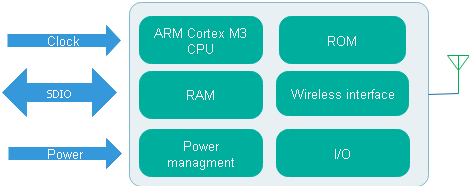
You may already be familiar with these from configuring a serial link, or network hardware; they provide a programming interface into a vendor-specific driver. Since the BCM/CTW43xxx chips are intelligent (they have their own CPU) the IOCTL calls are handled directly by the firmware we’ve programmed into the chip. So even though we’re in ‘bare metal’ mode, without an operating system, we still need to handle IOCTLs.

The IOCTL calls are listed in the wwd_wlioctl.h in WICED or WiFi Host Driver, or wlioctl_defs.h, and there are over 300 of them; this post will concentrate on the code that sends IOCTL requests and handles the responses, and we’ll check they are working by doing a quick network scan – more interesting things, like transmission & reception, will have to wait for the next part.

Message structure

When using IOCTL calls, you are essentially writing a data packet to the WiFi RAM, waiting for an acknowledgement, then reading back the response. As you’d expect, there is a specific data format for the requests and responses, though it does have some strange features:

#define IOCTL_MAX_DLEN  256

typedef struct {
    uint8_t  seq,       // sdpcm_sw_header
             chan,
             nextlen,
             hdrlen,
             flow,
             credit,
             reserved[2];
    uint32_t cmd;       // CDC header
    uint16_t outlen,
             inlen;
    uint32_t flags,
             status;
    uint8_t data[IOCTL_MAX_DLEN];
} IOCTL_CMD;

typedef struct {
    uint16_t len;
    uint8_t  reserved1,
             flags,
             reserved2[2],
             pad[2];
} IOCTL_GLOM_HDR;

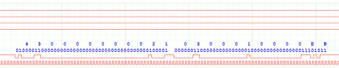
The best feature of the IOCTL data is that it always starts with a 16-bit length word, followed by the bitwise inverse of that length (least-significant byte first). For example, here is the decode of a request to set a variable ‘bus:rxglom’ to a value of 1:

19.290643 * Cmd 53 A500002C Wr WLAN 08000 len 44
19.290669 * Rsp 53 00001000 Flags 10
  Data  44 bytes: 2b 00 d4 ff 00 00 00 0c 00 00 00 00 07 01 00 00 0f 00 00 00 02 00 02 00 00 00 00 00 62 75 73 3a 72 78 67 6c 6f 6d 00 01 00 00 00 00 *
 IOC_W  44 bytes: seq=0 chan=0 nextlen=0 hdrlen=C flow=0 credit=0 cmd=107 outlen=F inlen=0 flags=20002 status=0 set 'bus:rxglom'
19.290769   Ack 2F FF

You can check this is an IOCTL message by adding the first two bytes to the second two: 002B + FFD4 = FFFF. It uses a command 53 to send a 44-byte request (actually 43 bytes, rounded up to nearest 4-byte value) to the RAD function, containing a header of mostly zeros with an IOCTL number of 107 hex (263 decimal) to set a variable, a null-terminated variable name, then the binary value.

It is then necessary to poll the WiFi chip to check when the response is available, and if so, acknowledge it:

19.291055 * Cmd 53 15404004 Rd BAK  180000:A020 len 4
  Data   4 bytes: 40 00 80 00 *
19.291081 * Rsp 53 00001000 Flags 10
19.291179 * Cmd 53 95404004 Wr BAK  180000:A020 len 4
19.291205 * Rsp 53 00001000 Flags 10
  Data   4 bytes: 40 00 00 00 *
19.291259   Ack 28 3F

The value of 40 hex in backplane register 2020 (A020 for a 32-bit value) shows there is a response, which is acknowledged by writing 40 hex to that register, then the response is read:

19.291377 * Cmd 53 21000040 Rd WLAN 08000 len 64
19.291403 * Rsp 53 00001000 Flags 10
  Data  64 bytes: 2b 00 d4 ff 02 00 00 0c 00 11 00 00 07 01 00 00 0f 00 00 00 00 00 02 00 00 00 00 00 62 75 73 3a 72 78 67 6c 6f 6d 00 01 00 00 00 00 00 00 00 00 00 00 00 00 00 00 00 00 00 00 00 00 00 00 00 00 *
 IOC_R  64 bytes: seq=2 chan=0 nextlen=0 hdrlen=C flow=0 credit=11 cmd=107 outlen=F inlen=0 flags=20000 status=0 set 'bus:rxglom'

The response is the same length as the request, and when writing to a variable it is largely a copy of the command. When receiving the response, it is important to check that it matches the request, as the two can easily get out of step. Unfortunately the sequence number can’t be used for this purpose (in this example the response is 2, and request is 0) instead the most-significant 16 bits of the ‘flags’ are a ‘request ID’ that should be the same for request & response, while the lower 16 bits are set to 2 for a write cycle, 0 for a read.

Equally strange is that the command length always seems to be the same as the response, so for a short command with a long response (such as ‘ver’) the command is 296 bytes long, just to carry a 3-character name. This is a bit crazy; sometime I’ll experiment with the header fields to see if there is a way round it.

Glom

I’ll admit this word wasn’t in my vocabulary until I encountered it in the WiFi drivers, and I’m still not entirely clear what it means. The transaction above sets ‘rxglom’ to 1, which enables ‘glom’ mode for incoming commands (‘rx’ refers to the WiFi chip command reception, not the host).

After this is set, another header is introduced into commands sent to the WiFi chip; I have accommodated this using another structure, and a union to cover both.

typedef struct {
    uint16_t len;
    uint8_t  reserved1,
             flags,
             reserved2[2],
             pad[2];
} IOCTL_GLOM_HDR;

typedef struct {
    IOCTL_GLOM_HDR glom_hdr;
    IOCTL_CMD  cmd;
} IOCTL_GLOM_CMD;

typedef struct
{
    uint16_t len,           // sdpcm_header.frametag
             notlen;
    union 
    {
        IOCTL_CMD cmd;
        IOCTL_GLOM_CMD glom_cmd;
    };
} IOCTL_MSG;

The good news is that the first 4 bytes of any message remain the same (16-bit length, and its bitwise inverse); the bad news is that the new header is shoehorned in after that, pushing the other headers out by 8 bytes.

Here is an example: getting ‘cur_ethaddr’ which is the 6-byte MAC address:

19.291837 * Cmd 53 A5000038 Wr WLAN 08000 len 56
19.291863 * Rsp 53 00001000 Flags 10
  Data  56 bytes: 38 00 c7 ff 34 00 00 01 00 00 00 00 01 00 00 14 00 00 00 00 06 01 00 00 14 00 00 00 00 00 03 00 00 00 00 00 63 75 72 5f 65 74 68 65 72 61 64 64 72 00 00 00 00 00 00 00 *
 IOC_W  56 bytes: seq=1 chan=0 nextlen=0 hdrlen=14 flow=0 credit=0 cmd=106 outlen=14 inlen=0 flags=30000 status=0 get 'cur_etheraddr'
19.291973   Ack 2F FF

I’m sure there must be some point to the extended header, but right now I’m not at all sure what it is. There doesn’t seem to be any official marker in the glom header to show that it has been included, which makes life difficult for any software attempting to decode the IOCTLs. For the time being, I’m hedging my bets by using a global variable to enable or disable this option, and leaving it disabled; hopefully its true purpose will be clear soon.

Partial data read

If the IOCTL command has a long response, and the software doesn’t read it all, the remainder will still be available for the next read. This can be demonstrated by the version (‘ver’) command; even though it is sent as a single 296-byte block, the Linux driver receives it as one block of 64 bytes, then another of 224:

19.295186 * Cmd 53 A5000128 Wr WLAN 08000 len 296
19.295212 * Rsp 53 00001000 Flags 10
  Data 296 bytes: 28 01 d7 fe 24 01 00 01 00 00 00 00 03 00 00 14 00 00 00 00 06 01 00 00 04 01 00 00 00 00 05 00 00 00 00 00 76 65 72 00 76 65 72 00 00 ..and so on..
 IOC_W 296 bytes: seq=3 chan=0 nextlen=0 hdrlen=14 flow=0 credit=0 cmd=106 outlen=104 inlen=0 flags=50000 status=0 get 'ver'
19.295583   Ack 2F FF
19.295980 * Cmd 52 00000A00 Rd BUS  00005
19.296006 * Rsp 52 00001002 Flags 10 data 02
19.296178 * Cmd 53 15404004 Rd BAK  180000:A020 len 4
  Data   4 bytes: 40 00 80 00 *
19.296204 * Rsp 53 00001000 Flags 10
19.296321 * Cmd 53 95404004 Wr BAK  180000:A020 len 4
19.296347 * Rsp 53 00001000 Flags 10
  Data   4 bytes: 40 00 00 00 *
19.296404   Ack 28 3F
19.296563 * Cmd 53 21000040 Rd WLAN 08000 len 64
19.296589 * Rsp 53 00001000 Flags 10
  Data  64 bytes: 20 01 df fe 05 00 00 0c 00 14 00 00 06 01 00 00 04 01 00 00 00 00 05 00 00 00 00 00 77 6c 30 3a 20 4f 63 74 20 32 33 20 32 30 31 37 20 30 33 3a 35 35 3a 35 33 20 76 65 72 73 69 6f 6e 20 37 2e *
 IOC_R  64 bytes: seq=5 chan=0 nextlen=0 hdrlen=C flow=0 credit=14 cmd=106 outlen=104 inlen=0 flags=50000 status=0 get 'wl0: Oct 23 2017 03:55:53 version 7.'
19.296841 * Cmd 53 210000E0 Rd WLAN 08000 len 224
19.296867 * Rsp 53 00001000 Flags 10
  Data 224 bytes: 34 35 2e 39 38 2e 33 38 20 28 72 36 37 34 34 34 32 20 43 59 29 20 46 57 49 44 20 30 31 2d 65 35 38 64 32 31 39 66 0a 00 00 ..and so on..

This serves to emphasise the important of reading all the data from every response, and checking that the Request ID matches that of the response; it’d be all to easy for the network driver to lose track.

Events

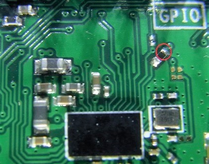
So far, we’ve dealt had a strict one-to-one matching between request and response, but how does the WiFi chip indicate when it has extra data available? For example, a single network scan may generate 10 or 20 data blocks (one for every access point), how does the host know when this data is available? There is mention of an interrupt pin (which we’ll save for a future blog) but how can the driver software check for data pending?

I puzzled over this for some time, on the assumption there must be a special register to indicate this, but in the end it seems that the driver just issues a normal data read; if data is available it can be recognised by the length header, if not zeros are returned.

The WiFi chip has a finite amount of buffer space to queue up such events; this is the ‘credit’ value in the IOCTL header; presumably the network driver should check this to see if events have been lost due to running out of buffers.

Network scan

Finally, we get to do something vaguely useful; scan for WiFi networks. There are 2 types: ‘iscan’ and ‘escan’. The first is an incremental scan, that seems easier to use, but is marked as ‘deprecated’ in some source code. The second is supposed to be more versatile (i.e. more complicated) but is the preferred option, so that is what we’ll be using.

We need to fill in a structure with the scan parameters; due to the large number of networks in the vicinity, I usually scan a single channel:

// WiFi channel number to scan (0 for all channels)
#define SCAN_CHAN       1

typedef struct {
    uint32_t version;
    uint16_t action,
             sync_id;
    uint32_t ssidlen;
    uint8_t  ssid[32],
             bssid[6],
             bss_type,
             scan_type;
    uint32_t nprobes,
             active_time,
             passive_time,
             home_time;
    uint16_t nchans,
             nssids;
    uint8_t  chans[14][2],
             ssids[1][32];
} SCAN_PARAMS;

SCAN_PARAMS scan_params = {
    .version=1, .action=1, .sync_id=0x1234, .ssidlen=0, .ssid={0}, 
    .bssid={0xff,0xff,0xff,0xff,0xff,0xff}, .bss_type=2, .scan_type=1, 
    .nprobes=~0, .active_time=~0, .passive_time=~0, .home_time=~0, 
#if SCAN_CHAN == 0
    .nchans=14, .nssids=0, 
    .chans={{1,0x2b},{2,0x2b},{3,0x2b},{4,0x2b},{5,0x2b},{6,0x2b},{7,0x2b},
      {8,0x2b},{9,0x2b},{10,0x2b},{11,0x2b},{12,0x2b},{13,0x2b},{14,0x2b}},
#else
    .nchans=1, .nssids=0, .chans={{SCAN_CHAN,0x2b}}, .ssids={{0}}
#endif
};

The scan is triggered by sending this data in an ‘escan’ IOCTL call, but first we must tell the chip that we’re interested in the response events. This is done by sending a very large bitfield, with a bit set for each event you want to receive; there are over 140 possible events, so you need to pick the right one. I got the list from whd_events_int.h which is part of the Cypress WiFi Host Driver project; if you don’t know what that is, please refer to part 1 of this blog, which describes all the resources I’m using.

So the code to trigger the scan becomes:

#define EVENT_ESCAN_RESULT  69
#define EVENT_MAX           160
#define SET_EVENT(e)        event_msgs[e/8] = 1 << (e & 7)
uint8_t event_msgs[EVENT_MAX / 8];

SET_EVENT(EVENT_ESCAN_RESULT);
ioctl_set_data("event_msgs", event_msgs, sizeof(event_msgs));
ioctl_set_data("escan", &scan_params, sizeof(scan_params));

Surprisingly easy, until we get back the results of the scan, which has one varying-length record for every WiFi access point found. There is a lot of data, around 300 to 600 bytes per record, so we need to do some heavyweight decoding.

Decoding the scan data

So far, I’ve avoided including any of the standard Cypress / Broadcom header files in my project. This is because any one header file often depends on another 2, which then depends on another 5, and so on… Quite rapidly, you’re including a large chunk of the Operating System which isn’t at all necessary; it just makes the decoding process much harder to follow.

Fortunately for this project, there is a way to avoid these major OS dependencies; use header files that were created for use in embedded systems, namely the Cypress WiFi Host Driver described in part 1 of this blog. Here are the structures that are needed for decoding the scan response data, and the files they’re in:

whd_types.h:
	whd_security, whd_scan_type, whd_bss_type, whd_802_11_band, whd_mac, whd_ssid, whd_bss_type, 
	whd_event_header [-> whd_event_msg], wl_bss_info
whd_events.h:
	whd_event_ether_header, whd_event_eth_hdr, whd_event_msg, whd_event
whd_wlioctl.h:
	wl_escan_result

Additional dependencies for these files are in:

cy_result.h, cyhal_hw_types.h, whd.h

So only 6 extra files need to be included at this stage, and we’ve avoided the unnecessary complexity of an Operating System interface – after all, this driver is supposed to be bare-metal code.

The code to print the MAC address, channel number and SSID (network name) is:

// Escan result event (excluding 12-byte IOCTL header)
typedef struct {
    uint8_t pad[10];
    whd_event_t event;
    wl_escan_result_t escan;
} escan_result;

escan_result *erp = (escan_result *)eventbuff;

n = ioctl_get_event(eventbuff, sizeof(eventbuff));
if (n > sizeof(escan_result))
{
    printf("%u bytes\n", n);
    disp_mac_addr((uint8_t *)&erp->event.whd_event.addr);
    printf(" %2u ", SWAP16(erp->escan.bss_info->chanspec));
    disp_ssid(&erp->escan.bss_info->SSID_len);
}

The scan result data fields are in network-standard byte-order (big endian) so the channel number needs to be byte-swapped.

Running the code

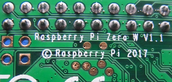
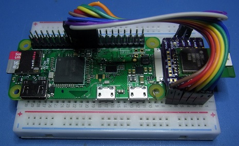
If you want to try out the code so far, you’ll need a Pi ZeroW with a USB-serial cable attached, the arm-none-eabi-gcc compiler and gdb debugger. You can find full details and a simple test program here; it is worth running this before attempting the Zerowi project.

The source code is at https://github.com/jbentham/zerowi, ‘make_scan.bat’ will create zerowi.elf on windows, which is downloaded into the target using the ‘run’ batch file. This executes alpha_speedup.py to accelerate the serial link from 115200 to 921600 baud, then runs Arm gdb using the setup commands in run.gdb.

I have provided Linux scripts ‘make_scan’ and ‘run’, these need to be made executable using ‘chmod +x’. The Alpha debugger does require arm-none-eabi-gdb, which isn’t included in many Linux distributions (including Raspbian Buster) so may need to be built from source.

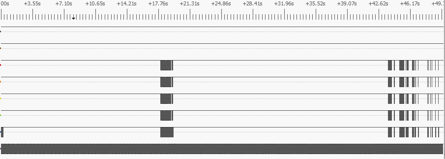
My Windows system uses serial port COM7, and Linux uses /dev/ttyUSB0; yours may well be different, so you’ll need to change scripts accordingly. If the Cypress firmware is included in the build image (i.e. ‘INCLUDE_FIRMWARE’ is non-zero) then it will take around 10 seconds to load the executable image onto the ZeroW. When the code runs you should see a list of access points; to keep the number of entries low, I only scan a single channel, by default channel 1:

360 bytes
7A:30:D9:96:DA:xx  1 BTWifi-X
460 bytes
84:A4:23:04:81:xx  1 PLUSNET
360 bytes
BC:30:D9:96:DA:xx  1 BTHub6
456 bytes
20:E5:2A:0E:A1:xx  1 Virginia Drive
312 bytes
7A:30:D9:96:DA:xx  1 BTWifi-with-FON
312 bytes
00:1D:AA:C1:75:xx  1 testnet

The last of the these is a special test network I’ll be using in subsequent parts of this blog.

To select another channel, change SCAN_CHAN at the top of zerowi.c; if set to zero, all channels will be scanned.

[Overview] [Previous part] [Next part]

Copyright (c) Jeremy P Bentham 2020. Please credit this blog if you use the information or software in it.

In the previous post we sent some commands to the WiFi chip, and got a response. To make the chip do anything useful, we need to program its internal CPU, as it doesn’t have code in ROM.

It does have configuration tables in ROM, that indicate what resources it possesses, and their locations, so the chip variants can all be programmed by a single driver. However, parsing these tables isn’t easy; the simplest code I’ve found is in the the Plan9 driver (see part 1 of this blog for details), and that is moderately impenetrable; here is the parser output for the ZeroW (values in hex):

chip ID A9A6 hex, 43430 decimal
coreid 800, corerev 31
  chipcommon 18000000
coreid 812, corerev 27
  d11ctl 18101000
coreid 829, corerev 15
  sdregs 18002000
  sdiorev 15
coreid 82a, corerev 9
  armcore 82a (ARMcm3)
  armregs 18003000
coreid 80e, corerev 16
  socramregs 18004000

I think these are the Intellectual Property (IP) cores within the chip, and the locations they occupy in the memory map, but in the absence of documentation, a lot of guesswork is required. So I decided to ignore the configuration tables, and just use the same addresses as the Linux driver, after it has done the decode. This makes my driver a lot less flexible, as the addresses will have to be changed for each new chip, but there aren’t many of them, so only a handful of definitions will need changing.

The most important number is the chip ID; it should be A9A6 hex, so it’d be a good idea to check our chip matches that. In part 3 my code did some preliminary SDIO initialisation, now to follow on from that:

// SD function numbers
#define SD_FUNC_BUS     0
#define SD_FUNC_BAK     1
#define SD_FUNC_RAD     2

// Maximum block sizes
#define SD_BAK_BLK_BYTES    64
#define SD_RAD_BLK_BYTES    512

// [0.243831] Set bus interface
sdio_cmd52_writes(SD_FUNC_BUS, BUS_SPEED_CTRL_REG, 0x03, 1);
sdio_cmd52_writes(SD_FUNC_BUS, BUS_BI_CTRL_REG, 0x42, 1);
// [17.999101] Set block sizes
sdio_cmd52_writes(SD_FUNC_BUS, BUS_BAK_BLKSIZE_REG, SD_BAK_BLK_BYTES, 2);
sdio_cmd52_writes(SD_FUNC_BUS, BUS_RAD_BLKSIZE_REG, SD_RAD_BLK_BYTES, 2);

The SD function numbers allow Command 52 & 53 to access 3 different interfaces within the chip: think ‘hardware functions’ rather than ‘software functions’. The SDIO bus interface is configured using the ‘bus’ function, and is set into high-speed mode (as discussed in part 2). Then the block sizes for the backplane (‘BAK’) and radio (‘RAD’) functions are set; these are limited to 64 & 512 bytes by the hardware. These will be used by command 53 when operating in multi-block mode.

#define BAK_BASE_ADDR           0x18000000              // CHIPCOMMON_BASE_ADDRESS

// [17.999944] Enable I/O 
sdio_cmd52_writes(SD_FUNC_BUS, BUS_IOEN_REG, 1<<SD_FUNC_BAK, 1);
if (!sdio_cmd52_reads_check(SD_FUNC_BUS, BUS_IORDY_REG, 0xff, 2, 1))
    log_error(0, 0);
// [18.001750] Set backplane window
sdio_bak_window(BAK_BASE_ADDR);
// [18.001905] Read chip ID 
sdio_cmd53_read(SD_FUNC_BAK, SB_32BIT_WIN, u32d.bytes, 4);

We now use the ‘bus’ function to enable the ‘backplane’ interface; by default, the IP cores in the chip are switched off to conserve power, and they need to be enabled; the second line of code checks that the core has actually powered up (I/O enabled -> I/O ready). Once the backplane function is enabled, we set a window pointing to the common base address (‘chipcommon’ in the Plan9 driver) then do a read, and we get hex values A6 A9 41 15, which is correct. However, some explanation is needed with regard to the backplane window.

Backplane window

You may recall that the commands we’re using here, CMD52 and CMD53, only have a 17-bit address range, yet the chip uses 32-bit addresses internally. The way this is handled is by writing a 24-bit value to 3 of the backplane registers, to act as an offset within the internal space.

// Backplane window
#define SB_32BIT_WIN    0x8000
#define SB_ADDR_MASK    0x7fff
#define SB_WIN_MASK     (~SB_ADDR_MASK)

// Set backplane window, don't set if already OK
void sdio_bak_window(uint32_t addr)
{
    static uint32_t lastaddr=0;
    
    addr &= SB_WIN_MASK;
    if (addr != lastaddr)
        sdio_cmd52_writes(SD_FUNC_BAK, BAK_WIN_ADDR_REG, addr>>8, 3);
    lastaddr = addr;
}
// Do 1 - 4 CMD52 writes to successive addresses
int sdio_cmd52_writes(int func, int addr, uint32_t data, int nbytes)
{
    int n=0;

    while (nbytes--)
    {
        n += sdio_cmd52(func, addr++, (uint8_t)data, SD_WR, 0, 0);
        data >>= 8;
    }
    return(n);
}

It is important to realise that this is a simple windowing scheme where the bottom 15 bits are provided by the offset, and the top 17 bits by the window: the two values aren’t added together. An additional complication (yes, really) is that there are 2 copies of the lower 15-byte address space; 0 – 7fff hex is for byte accesses, and 8000 – ffff hex is for 32-bit word accesses (offset SB_32BIT_WIN).

To give a concrete example, here is the analysis of the RPi driver fetching the CPU ID:

18.001455 * Cmd 52 92001400 Wr BAK  1000A 00
18.001481 * Rsp 52 00001000 Flags 10 data 00
18.001618 * Cmd 52 92001600 Wr BAK  1000B 00
18.001644 * Rsp 52 00001000 Flags 10 data 00
18.001750 * Cmd 52 92001818 Wr BAK  1000C 18 Bak Win 180000
18.001777 * Rsp 52 00001018 Flags 10 data 18
18.001905 * Cmd 53 15000004 Rd BAK  180000:8000 len 4
  Data   4 bytes: a6 a9 41 15 *

You can see the 3 CMD52 write cycles to set the window address, then the 4-byte read cycle, with the offset into the 32-bit area. The ‘win 180000’ and ‘180000:8000’ labels are my analysis code trying to be helpful, by saving the window value, and repeating it at the subsequent read cycle.

Firmware file

There are various firmware versions that could be used (see Cypress WICED) but I’m using the same version as the RPi driver, available here. It is around 300K bytes; eventually, it’ll be stored in the SD card filesystem, but for the time being I wanted a simpler storage mechanism, so attached an external SPI memory device, that can be programmed by a standard RPi utility, and is really easy to read back.

This extra hardware isn’t compulsory; there is an INCLUDE_FIRMWARE option in the source code to link the firmware file into the binary image; the functionality is the same, it just takes longer to load over the target serial link.

The device I used is an EN25Q80B, which has a megabyte of serial flash memory. MikroElektronika sell a small flash click board that is simple to connect to the ZeroW, as follows:

MicroE pi   RPi pin
Gnd          25
3V3          17
SDI          19
SDO          21
SCK          23
CS           24

This can be programmed using the following utilities that are included in the standard Linux distribution:

objcopy -F binary brcmfmac43430-sdio.bin flash.bin --pad-to 0x100000
sudo apt install flashrom
sudo modprobe spi_bcm2835
flashrom -p linux_spi:dev=/dev/spidev0.0,spispeed=1000 -w flash.bin

The version of flashrom I used does issue a warning that the Eon chip isn’t fully supported, but still programs it OK. Reading the chip is really easy:

#define SPI0_BASE       (REG_BASE + 0x204000)
#define SPI0_CS         (uint32_t *)SPI0_BASE
#define SPI0_FIFO       (uint32_t *)(SPI0_BASE + 0x04)
#define SPI0_CLK        (uint32_t *)(SPI0_BASE + 0x08)
#define SPI0_DLEN       (uint32_t *)(SPI0_BASE + 0x0c)
#define SPI0_DC         (uint32_t *)(SPI0_BASE + 0x14)

#define SPI0_CE0_PIN    8
#define SPI0_MISO_PIN   9
#define SPI0_MOSI_PIN   10
#define SPI0_SCLK_PIN   11

// Initialise flash interface (SPI0)
void flash_init(int khz)
{
    gpio_set(SPI0_CE0_PIN, GPIO_ALT0, GPIO_NOPULL);
    gpio_set(SPI0_MISO_PIN, GPIO_ALT0, GPIO_PULLUP);
    gpio_set(SPI0_MOSI_PIN, GPIO_ALT0, GPIO_NOPULL);
    gpio_set(SPI0_SCLK_PIN, GPIO_ALT0, GPIO_NOPULL);
    *SPI0_CS = 0x30;
    *SPI0_CLK = CLOCK_KHZ / khz;
}

// Set / clear SPI chip select
void spi0_cs(int set)
{
    *SPI0_CS = set ? *SPI0_CS | 0x80 : *SPI0_CS & ~0x80;
}

// Start a flash read cycle (EN25Q80 device)
void flash_open_read(int addr)
{
    uint8_t rxdata[4], txdata[4]={3, (uint8_t)(addr>>16), (uint8_t)(addr>>8), (uint8_t)(addr)};
    
    spi0_cs(1);
    spi0_xfer(txdata, rxdata, 4);
}
// Read next block
void flash_read(uint8_t *dp, int len)
{
    while (len--)
    {
        *SPI0_FIFO = 0;
        while((*SPI0_CS & (1<<17)) == 0) ;
        *dp++ = *SPI0_FIFO;
    }
}
// End a flash cycle
void flash_close(void)
{
    spi0_cs(0);
}

If you don’t want to bother with this, just set the INCLUDE_FIRMWARE option in the source code, which links the firmware file into the main executable.

File upload

Before we can upload the code, there is a lot more initialisation to be done; another 34 commands that I won’t be describing here, mainly because I’m having difficulty understanding them in the absence of documentation; for now, the source code is the only explanation you’ll get.

The process of transferring the file is made a bit more complicated by the windowing scheme I described earlier; we have to move that along after every 32K. Command 53 is used in multi-block mode, so one command is issued for multiple data blocks.

// Upload blocks of firmware from flash to chip RAM
int write_firmware(void)
{
    int len, n=0, nbytes=0, nblocks;
    uint32_t addr;

    flash_open_read(0);
    while (nbytes < FIRMWARE_LEN)
    {
        addr = sdio_bak_addr(nbytes);
        len = MIN(sizeof(txbuffer), FIRMWARE_LEN-nbytes);
        nblocks = len / SD_BAK_BLK_BYTES;
		if (nblocks > 0)
        {
            flash_read(txbuffer, nblocks*SD_BAK_BLK_BYTES);
            n = sdio_write_blocks(SD_FUNC_BAK, SB_32BIT_WIN+addr, txbuffer, nblocks);
            if (!n)
                break;
            nbytes += nblocks * SD_BAK_BLK_BYTES;
        }
        else
        {
            flash_read(txbuffer, len);
            txbuffer[len++] = 1;
            sdio_cmd53_write(SD_FUNC_BAK, SB_32BIT_WIN+addr, txbuffer, len);
            nbytes += len;
        }
    }
    flash_close();
    return(nbytes);
}
// Write multiple 64-byte command 53 blocks (max 32K in total)
int sdio_write_blocks(int func, int addr, uint8_t *dp, int nblocks)
{
    int n=0;
    SDIO_MSG rspx, cmd={.cmd53 = {.start=0, .cmd=1, .num=53,
        .wr=1, .func=func, .blk=1, .inc=1, .addrh=(uint8_t)(addr>>15)&3,
        .addrm=(uint8_t)(addr>>7), .addrl=(uint8_t)(addr&0x7f),
        .lenh=(uint8_t)(nblocks>>8)&1, .lenl=(uint8_t)nblocks, .crc=0, .stop=1}};

    clk_0(1);
    add_crc7(cmd.data);
    log_msg(&cmd);
    sdio_cmd_write(cmd.data, MSG_BITS);
    if (sdio_rsp_read(rspx.data, MSG_BITS, SD_CMD_PIN))
    {
        gpio_write(SD_D0_PIN, 4, 0xf);
        gpio_mode(SD_D0_PIN, GPIO_OUT);
        gpio_mode(SD_D1_PIN, GPIO_OUT);
        gpio_mode(SD_D2_PIN, GPIO_OUT);
        gpio_mode(SD_D3_PIN, GPIO_OUT);
        while (n++ < nblocks)
        {
            sdio_block_out(dp, SD_BAK_BLK_BYTES);
            sdio_rsp_read(rspx.data, BLOCK_ACK_BITS, SD_D0_PIN);
            dp += SD_BAK_BLK_BYTES;
            clk_0(2);
        }
        gpio_mode(SD_D0_PIN, GPIO_IN);
        gpio_mode(SD_D1_PIN, GPIO_IN);
        gpio_mode(SD_D2_PIN, GPIO_IN);
        gpio_mode(SD_D3_PIN, GPIO_IN);
    }
    clk_0(1);
    return(n);
}

Once that is complete, we must load in the configuration data, which is available here. A small amount of pre-processing is required, namely removing the comment lines, and replacing all the newline characters with nulls. Since the file is small, command 53 is used in single-block mode.

// Upload blocks of config data to chip NVRAM
int write_nvram(void)
{
    int nbytes=0, len;

    sdio_bak_window(0x078000);
    while (nbytes < config_len)
    {
        len = MIN(config_len-nbytes, SD_BAK_BLK_BYTES);
        sdio_cmd53_write(SD_FUNC_BAK, 0xfd54+nbytes, &config_data[nbytes], len);
        nbytes += len;
    }
    return(nbytes);
}

After another 12 initialisation commands, we can check if the code was loaded OK:

usdelay(50000);
if (!sdio_cmd52_reads(SD_FUNC_BAK, BAK_CHIP_CLOCK_CSR_REG, &u32d.uint32, 1) || u32d.uint8!=0xd0)
    log_error(0, 0);
// [19.190728]
sdio_cmd52_writes(SD_FUNC_BAK, BAK_CHIP_CLOCK_CSR_REG, 0xd2, 1);
sdio_bak_write32(SB_TO_SB_MBOX_DATA_REG, 0x40000);
sdio_cmd52_writes(SD_FUNC_BUS, BUS_IOEN_REG, (1<<SD_FUNC_BAK) | (1<<SD_FUNC_RAD), 1);
sdio_cmd52_reads(SD_FUNC_BUS, BUS_IORDY_REG, &u32d.uint32, 1);
usdelay(100000);
if (!sdio_cmd52_reads(SD_FUNC_BUS, BUS_IORDY_REG, &u32d.uint32, 1) || u32d.uint8!=0x06)
    log_error(0, 0);

If the first value is D0 hex, and the second is 6, then all is well, and after another 21 initialisation commands, we can think about doing something useful with the chip…

[Overview] [Previous part] [Next part]

Copyright (c) Jeremy P Bentham 2020. Please credit this blog if you use the information or software in it.

This diagram shows the internals of the CYW43xxx chip in simplified form; the important point is that the chip has its own CPU, RAM and ROM; it is a computer-within-a-computer.

In part 2 I mentioned the lack of documentation, and now this becomes a major issue; how to program this complex chip, with no data on its internals. Cypress have partially solved this problem by issuing a standard binary ‘blob’ (roughly 300K bytes) that contains all the code for the embedded CPU; we’ll just be feeding data and control messages into that program, not knowing (or caring) what it is doing to the chip hardware.

I say the problem is ‘partially’ solved because we have to set up the chip to receive this program, upload the code into its RAM, then configure the chip to run it.. a sizeable task, as I’ve discovered.

First steps

The first task is to get the WiFi chip to respond to our commands. The SD and SDIO specifications offer plenty of flowcharts that describe how such a device might be initialised, but I had minimal success with these; they may be applicable to older chips, but maybe the later incarnations of the CYW43xxx just treat the SDIO bus as a convenient parallel interface, rather than slavishly following a specification that was designed for plug-in SD cards.

Then there are the timing issues; a quick glance at the existing code shows many instances where SDIO commands are artificially delayed; after you change something within the chip, it needs time to react before receiving the next command – and if that is sent too quickly, the chip just ignores it, with no error response.

The best way I could find to tackle these problems is to capture all the SDIO commands, responses & data when the Linux driver is running. The capture method is described in the previous part of this blog, and it results in a sizeable file: over 5 gigabytes as a CSV. It contains over 2,200 commands and 13,000 data blocks, so I wrote an application (‘sd_decoder’) to decode the file and display the commands. It turns out that there is a lot of redundancy (for example, the driver loads the 300K binary into the chip, then reads it all back again) so by focusing purely on one WiFi chip, we can make major simplifications.

Fragments of the simplified command sequence can then be replayed into the chip, and eventually, it starts to respond – the first time you get a response from a new chip is a happy day! Here are the first few commands the Linux driver uses to start up the chip:

 0.000331 74 00 00 0c 00 39 * Cmd 52 00000C00 Rd BUS  00006
 0.002759 74 80 00 0c 08 9f * Cmd 52 80000C08 Wr BUS  00006 08
 0.025217 40 00 00 00 00 95 * Cmd  0 00000000
 0.028130 48 00 00 01 aa 87 * Cmd  8 000001AA
 0.028527 45 00 00 00 00 5b * Cmd  5 00000000
 0.028660 3f 20 ff ff 00 ff ? Rsp 63 20FFFF00
 0.028875 45 00 20 00 00 3d * Cmd  5 00200000
 0.029007 3f a0 ff ff 00 ff ? Rsp 63 A0FFFF00
 0.029228 43 00 00 00 00 21 * Cmd  3 00000000
 0.029353 03 00 01 00 00 eb * Rsp  3 00010000
 0.029690 47 00 01 00 00 dd * Cmd  7 00010000
 0.029815 07 00 00 1e 00 a1 * Rsp  7 00001E00

To explain the format; firstly the time in seconds, then 6 command/response bytes, ‘*’ to indicate CRC is correct, or ‘?’ if incorrect, then a partial decode.

A few points to note:

• The first 4 commands produce no responses.
• There are jumps in the timestamp, presumably caused by intentional delays.
• CMD5 is described in the SDIO specification as enabling I/O mode, but the response we get has an incorrect CRC.
• The CMD3 – CMD7 sequence is described in the SD specification; it is the way that a host selects one card from multiple card slots; CMD3 gets a Relative Card Address (RCA), then command 7 selects the card using that address.

It’d be nice to understand why two of the commands have failed CRCs, but the Linux driver ignores that error, so I will as well. The above sequence is implemented in my code as follows:

int rca;
sdio_cmd52(SD_FUNC_BUS, 0x06, 0, SD_RD, 0, 0);   
usdelay(20000);
sdio_cmd52(SD_FUNC_BUS, 0x06, 8, SD_WR, 0, 0);   
usdelay(20000);
sdio_cmd(0, 0, 0);
sdio_cmd(8, 0x1aa, 0);
// Enable I/O mode
sdio_cmd(5, 0, 0);
sdio_cmd(5, 0x200000, 0);
// Assert SD device
sdio_cmd(3, 0, &resp);
rca = SWAP16(resp.rsp3.rcax);
sdio_cmd7(rca, 0);

Note the time delays; it is tempting to reduce them, but I have found from bitter experience that this can result in major problems much later on (as a critical setting has been ignored), so I wouldn’t recommend doing that.

Raspberry Pi I/O

Now it is necessary to translate the SDIO commands into hardware I/O cycles. The good news about bare-metal programming is that is isn’t necessary to use a fancy driver, or seek permission from the operating system; we can just control the I/O directly.

The primary source of information is the ‘BCM2835 ARM Peripherals’ document; armed with that and knowledge of the I/O base address (0x20000000 for the Pi ZeroW) we can create suitable low-level functions.

// Addresses
#define REG_BASE    0x20000000      // Pi Zero (0x3F000000 for Pi 3)
#define GPIO_BASE       (REG_BASE + 0x200000)
#define GPIO_MODE0      (uint32_t *)GPIO_BASE
#define GPIO_SET0       (uint32_t *)(GPIO_BASE + 0x1c)
#define GPIO_CLR0       (uint32_t *)(GPIO_BASE + 0x28)
#define GPIO_REG(a)     ((uint32_t *)a)

// Mode values
#define GPIO_IN         0
#define GPIO_OUT        1
#define GPIO_ALT0       4
#define GPIO_ALT1       5
#define GPIO_ALT2       6
#define GPIO_ALT3       7

// Configure pin as input or output
void gpio_mode(int pin, int mode)
{
    uint32_t *reg = GPIO_REG(GPIO_MODE0) + pin / 10;
    int shift = (pin % 10) * 3;

    *reg = (*reg & ~(7 << shift)) | (mode << shift);
}

// Set an O/P pin
void gpio_out(int pin, int val)
{
    uint32_t *reg = (val ? GPIO_REG(GPIO_SET0) : GPIO_REG(GPIO_CLR0)) + pin/32;

    *reg = 1 << (pin % 32);
}

// Get an I/P pin value
uint8_t gpio_in(int pin)
{
    uint32_t *reg = GPIO_REG(GPIO_LEV0) + pin/32;

    return (((*reg) >> (pin % 32)) & 1);
}

Configuring a pin as an input or output is done by setting a 3-bit values. Writing 1 or 0 to a pin is (sadly) done using separate set & clear registers; this does make any speed-optimisations (e.g. direct DMA to I/O ports) significantly harder, so I haven’t tried this yet.

Running under Linux

Although the whole purpose of this project is to run without Linux, after I’d written the above code, I did wonder whether it’d speed up development if I ran it under Linux with the WiFi interface shut down, using mmap() to gain access to the devices at low level.

This experiment failed; I never got reliable communications with the WiFi chip, and the operating system had a tendency to crash after my code was run. This isn’t too surprising, since the whole point of the OS is to control the hardware, and having a user-mode program controlling it as well, is really asking for trouble.

Timer

In addition to I/O cycles, we need a microsecond timing reference, that can be used to provide accurate delays. Fortunately there is a 32-bit register clocked at 1 MHz that is ideal for the purpose.

#define USEC_BASE       (REG_BASE + 0x3000)
#define USEC_REG()      ((uint32_t *)(USEC_BASE+4))

// Delay given number of microseconds
void usdelay(int usec)
{
    int ticks;

    ustimeout(&ticks, 0);
    while (!ustimeout(&ticks, usec)) ;
}

// Return non-zero if timeout
int ustimeout(int *tickp, int usec)
{
    int t = *USEC_REG();

    if (usec == 0 || t - *tickp >= usec)
    {
        *tickp = t;
        return (1);
    }
    return (0);
}

SDIO output

The Raspberry Pi CPU is sufficiently fast that we can easily toggle the clock line at 500 kHz, while shifting the command bits out.

#define SD_CLK_DELAY    1   // Clock on/off time in usec

// Write command to SD interface
void sdio_cmd_write(uint8_t *data, int nbits)
{
   uint8_t b, n;

    gpio_mode(SD_CMD_PIN, GPIO_OUT);
    for (n=0; n<nbits; n++)
    {
        if (n%8 == 0)
            b = *data++;
        gpio_out(SD_CMD_PIN, b & 0x80);
        b <<= 1;
        usdelay(SD_CLK_DELAY);
        gpio_out(SD_CLK_PIN, 1);
        usdelay(SD_CLK_DELAY);
        gpio_out(SD_CLK_PIN, 0);
    }
    gpio_mode(SD_CMD_PIN, GPIO_IN);
}

This code could be made much faster, by eliminating the delays. When writing the data output function I took a more aggressive approach to the timing; the transfers are error-free with a 2 MHz clock (8 Mbit/s of data) and could go faster with some optimisation.

Reception is a lot more tricky, handling command responses, data on CMD53 read-cycles, and acknowledgements on write-cycles. This requires multiple state-machines, triggered by the clock edges and ‘start’ bit detection; see the source code for details.

The 7- and 16-bit CRC calculations for commands & data have already been explained in part 2 of this blog.

[Overview] [Previous part] [Next part]

Copyright (c) Jeremy P Bentham 2020. Please credit this blog if you use the information or software in it.

Hardware

I’m starting this project with the Raspberry Pi ZeroW, which uses the Cypress WiFi chip CYW43438. It interfaces to the ARM processor using Secure Digital I/O (SDIO), which consists of the following signals:

• Clock (1 line, O/P from CPU)
• Command (1 line, I/O)
• Data (4 lines, I/O)

Later in this blog, I’ll be describing what these pins do, in case you are a newcomer to the strange world of SDIO.

The I/O bit numbers are defined in the DeviceTree file for the board:

sdio_pins {
    brcm,pins = <0x00000022 0x00000023 0x00000024 0x00000025 0x00000026 0x00000027>;
    brcm,function = <0x00000007>;
    brcm,pull = <0x00000000 0x00000002 0x00000002 0x00000002 0x00000002 0x00000002>;
    phandle = <0x00000019>;
};

The ‘pull’ settings show that pullup resistors are enabled for pin 23 to 27 hex (GPIO35 to 39), and an initial guess would be that these pins are the command and data, while 22 hex (GPIO34) is the clock.

The datasheet mentions a power-on signal, and a quick trawl on the Web suggests that this could be GPIO41, which must be high to power up the WiFi interface. There is also mention of a low-speed (32 kHz) clock that may be needed when waking up the chip from low-power mode; it turns out this is on GPIO43. This can be verified by dumping the I/O configuration registers when the WiFi interface is running:

  20300000: 0013D660 00017030 A5040030 353A0002 00001000 00000000 00000000 00000000
  20300020: 00000000 01FF0000 00000F02 000E0207 00000000 00FF0133 00FF0133 00000000

Each pin has a 3-bit mode value, that shows whether it being used for simple input, output, or is connected to an internal peripheral (ALT0 – 5). The values above can be decoded by referring to the ‘BCM2835 ARM Peripherals’ data sheet, but an easier way is to use the ‘pigs’ front-end for the PIGPIO library, thus:

sudo pigpiod   [load PIGPIO daemon]
pigs mg 34     [get mode of GPIO pin 34]
7              [returned value 7: pin is ALT3]
pigs mg 43     [get mode of GPIO pin 43]
4              [returned value 4: pin is ALT0]

Pins 34 to 39 are all set to ALT3, which is unhelpfully labelled in the BCM2835 datasheet as ‘reserved’; in reality this means they are connected to the (undocumented) Arasan SD controller. GPIO43 is configured as ALT0, which is the clock source GPCLK2, configured for 32.768 kHz.

Attaching a logic analyser

To understand what the Linux driver is doing, I need to attach a logic analyser to the SDIO bus. This isn’t easy on most boards; the interface runs very fast (up to 50 MHz) so the only means of attachment is by soldering onto extremely small surface-mount components, that can easily be damaged.

However, the Pi Zerow has some interesting pads on the underside.

Those 7 gold circles are clearly attached to some internal signals, since they have conductive holes (known as ‘vias’) to tracks on other layers. Also, they’re in the right area for the SDIO interface, and it is possible they’re needed for testing the WiFi/ Bluetooth interface after the PCB is assembled. Monitoring these signals with WiFi running proved that they do have almost all of the SDIO signals, aside from the most important one: the clock. Further probing suggested that the only way to pick up that signal is on the other side of the board at a resistor, but connecting to this point is tricky; you need good surface-mount soldering skills to avoid damaging the board.

The main problem with the logic analyser interface is the sheer volume of data that’ll be accumulated. The boot process takes around a minute, with sporadic activity on the SDIO interface; catching all that, with a data rate of 50 MHz, would require a very complicated and/or expensive setup. Fortunately, the Raspberry Pi has an ‘overclocking’ setting in the boot file config.txt, which sets the clock rate to be used when the OS requests 50 MHz. This doesn’t just speed up the interface; a value of 1 or 2 MHz can be used to slow it right down, e.g.

# Add to /boot/config.txt:
dtparam=sdio_overclock=2

This allows a lower-cost analyser to be used (see part 1 of this blog for details) – and surprisingly, the change doesn’t make a lot of difference to the boot-time, since there are long pauses in SDIO activity, where the OS is doing other things. This can be seen by zooming the analyser display out to the maximum, showing 50 seconds of data:

The bottom trace is the clock, the next is the command (CMD) line, then there are the 4 data lines. Despite the long periods with no activity, there is a lot going on: over 2,200 commands and 13,000 data blocks are being exchanged between the CPU and the WiFi chip.

SDIO protocol

If, like me, you have some experience of the Serial Peripheral Interface (SPI), you may expect SDIO to be similar, in that it uses a clock line to synchronise the sender & receiver; the rising edge of the clock indicates that the data is stable, and can be read by the receiver.

However, there are a few key differences:

• Bi-directional. All the lines, apart from the clock, are bi-directional; either side can drive them.
• Command and data lines. There are separate lines for commands and data, and the 4 data lines act as a 4-bit parallel bus.
• Start & end bits. Instead of the SPI chip-select, the data and command lines idle high, then go low to signal the start of a transfer; this is referred to as a ‘start bit’, and is a single bit-time with a value of zero. At the end of the transfer there is a single bit with a value of 1, an ‘end bit’.
• Format. The format of SDIO commands and responses is standardised, with specific meaning to the transferred bytes.

It is well worth reading the SDIO specification; at the time of writing, the latest version that is available from the SD Association is “SD Specifications Part E1, SDIO Simplified Specification Version 3.00”. For a few of the commands you need to refer back to the “SD Specifications Part 1 Physical Layer Simplified Specification”, for example:

This is SD command 3 (generally abbreviated to CMD3) and response 6 (R6) from the target (WiFi chip). Both are specified at being 48 bits long, and you can see they begin with a 0 start-bit, and finish with a 1 end-bit. Between the two, the command line is briefly idle. It is a bit confusing that the reply to a command 3 is not a response 3; this is because there are a lot of commands (over 50) but many of them share the same response format, so only 7 possible responses have been defined.

The most common commands used in the SDIO interface are CMD52 and 53. Command 52 is used to read or write a single 8-bit value, while CMD53 transfers blocks of data, either singly or in batches. The following trace shows command 53 reading a single block of 4 data bytes; the command and response look similar to command 52, but there is also activity on the data lines, starting with a 4-bit value of zero, and ending with F hex.

SDIO interface code

In the absence of the necessary documentation, writing code for the ‘Arasan’ SD controller on the Raspberry Pi would be quite fraught, so I decided to use direct control (‘bit-bashing’ or ‘bit-banging’) of the I/O lines. The more experienced among you might be thinking this is a really bad idea, as it can be very CPU-intensive and slow, but I believe that the end-result (for example, booting the WiFi chip from scratch in 1 second) vindicates my decision – and if you want to use the controller, you can modify my code to do so.

The bit-patterns within the SDIO commands and responses are quite complex, and the code I’ve seen makes heavy use of bit-masking and shifting to combine the individual values into a single message. I’m not a fan of this approach, and prefer to use C language bitfields. For example, CMD52 has the following fields in the 6-byte message:

Start:             1 bit  (always 0)
Direction:         1 bit  (1 for command, 0 for response)
Command index:     6 bits (52 decimal for command 52)
R/W flag:          1 bit  (0 for read, 1 for write)
Function number:   3 bits (select the bus, backplane or radio interface)
RAW flag:          1 bit  (1 to read back result of write)
Unused:            1 bit
Register address: 17 bits (128K address space)
Unused:            1 bit
Data value:        8 bits (byte to be written, unused if read cycle)
CRC:               7 bits (cyclic redundancy check)
End:               1 bit  (always 1)

You’ll see that the values don’t all line up on convenient 8-bit boundaries; furthermore the data sheet defines the values with most-significant value first, whereas standard C structures have least-significant first.

My solution is to use macros to reverse the order of bits in the byte, so the command structure looks similar to the specification. These are used to create structures for the commands and responses, which are combined in a union.

#define BITF1(typ, a)             typ a
#define BITF2(typ, a, b)          typ b, a
#define BITF3(typ, a, b, c)       typ c, b, a
..and so on..

typedef struct
{
    BITF3(uint8_t,  start:1, cmd:1,   num:6);
    BITF5(uint8_t,  wr:1,    func:3,  raw:1, x1:1, addrh:2);
    BITF1(uint8_t,  addrm);
    BITF2(uint8_t,  addrl:7, x2:1);
    BITF1(uint8_t,  data);
    BITF2(uint8_t,  crc:7,   stop:1);
} SDIO_CMD52_STRUCT;

typedef union 
{
    SDIO_CMD52_STRUCT   cmd52;
    SDIO_RSP52_STRUCT   rsp52;
    SDIO_CMD53_STRUCT   cmd53;
    uint8_t             data[MSG_BYTES+2];
} SDIO_MSG;

The code to split the 17-bit address into 3 bytes is still a bit messy, but the structure definition does simplify the process of creating a command:

// Send SDIO command 52, get response, return 0 if none
int sdio_cmd52(int func, int addr, uint8_t data, int wr, int raw, SDIO_MSG *rsp)
{
    SDIO_MSG cmd={.cmd52 = {.start=0, .cmd=1, .num=52,
        .wr=wr, .func=func, .raw=raw, .x1=0, .addrh=(uint8_t)(addr>>15 & 3),
        .addrm=(uint8_t)(addr>>7 & 0xff), .addrl=(uint8_t)(addr&0x7f), .x2=0,
        .data=data, .crc=0, .stop=1}};

    return(sdio_cmd_rsp(&cmd, rsp));
}

For speed, the CRC is created using a byte-wide lookup table in RAM, which is computed on startup:

#define CRC7_POLY    (uint8_t)(0b10001001 << 1)

uint8_t crc7_table[256];

// Initialise CRC7 calculator
void crc7_init(void)
{
    for (int i=0; i<256; i++)
        crc7_table[i] = crc7_byte(i);
}

// Calculate 7-bit CRC of byte, return as bits 1-7
uint8_t crc7_byte(uint8_t b)
{
    uint16_t n, w=b;

    for (n=0; n<8; n++)
    {
        w <<= 1;
        if (w & 0x100)
            w ^= CRC7_POLY;
    }
    return((uint8_t)w);
}

// Calculate 7-bit CRC of data bytes, with l.s.bit as stop bit
uint8_t crc7_data(uint8_t *data, int n)
{
    uint8_t crc=0;

    while (n--)
        crc = crc7_table[crc ^ *data++];
    return(crc | 1);
}

Data CRC

The data transfer includes a CRC for every line, for example this is the transfer of the 4 bytes A6, A9, 41, and 15 hex.

A total of 12 bytes are transferred, because each data line has an added 16-bit CRC. This was a bit of a headache, since splitting the 4-bit data into individual 1-bit values for CRC calculation would considerably slow down the command generation & checking. Fortunately there is a easy way to calculate & check the CRC for each line, while still keeping the 4 values together. This comes from the realisation that the exclusive-or operation in the CRC doesn’t care what order the bits are in; we can rearrange the bits to match our data. So we can compute all 4 CRCs using a single 64-bit value:

Bit 0: bit 0 of 1st CRC
Bit 1: bit 0 of 2nd CRC
Bit 2: bit 0 of 3rd CRC
Bit 3: bit 0 of 4th CRC
Bit 4: bit 1 of 1st CRC
..and so on, up to..
Bit 63: bit 15 of 4th CRC

Once they have been computed, the 4 CRCs are transmitted by just shifting out the next 4 bits of the 64-bit value. To speed up the calculation, a 4-bit lookup table is initialised on startup:

#define CRC16R_POLY  (1<<(15-0) | 1<<(15-5) | 1<<(15-12))

uint64_t qcrc16r_poly, qcrc16r_table[16];

// Initialise bit-reversed CRC16 lookup table for 4-bit values
void qcrc16r_init(void)
{
    qcrc16r_poly = quadval(CRC16R_POLY);
    for (int i=0; i<(1<<SD_DATA_PINS); i++)
        qcrc16r_table[i]  = (i & 8 ? qcrc16r_poly<<3 : 0) |
                            (i & 4 ? qcrc16r_poly<<2 : 0) |
                            (i & 2 ? qcrc16r_poly<<1 : 0) |
                            (i & 1 ? qcrc16r_poly<<0 : 0);
}

// Spread a 16-bit value to occupy 64 bits
uint64_t quadval(uint16_t val)
{
    uint64_t ret=0;

    for (int i=0; i<16; i++)
        ret |= val & (1<<i) ? 1LL<<(i*4) : 0;
    return(ret);
}

Now when transmitting, the 64-bit (i.e. 4 x 16-bit) CRC is updated with every 4-bit value:

uint64_t qcrc=0;

// For each 4-bit value 'd':
qcrc = (qcrc >> 4) ^ qcrc16r_table[(d ^ (uint8_t)qcrc) & 0xf];

After the data has been sent, the CRC values are transmitted:

for (n=0; n<16; n++)
{
    output((uint8_t)qcrc & 0xf);
    qcrc >>= 4;
}

Bulk transfers

Command 53 can be used to transfer a single block (where the block size is specified in the command) or multiple blocks (where the block size has previously been set, and the number of blocks is specified in the command).

If the CPU is sending a single command, then writing multiple blocks to the WiFi chip, how does it check that the blocks are being received and processed OK? The answer is that when writing blocks, the recipient generates a brief acknowledgement back. Here is an example of a CMD53 write.

It is a bit difficult to see what is going on; the command and response are similar to all the others, but then (after a surprisingly long pause) the data is transferred from the CPU to the WiFi chip. Zooming in on that data:

4 bytes with the values 3, 0, 0, 0, are being transferred, then 8 bytes of CRC. However, after that, the recipient acknowledges the received data by driving the least-significant data line with a bit value of 00101000 00111111 (28 3F hex). To be honest, I haven’t been able to find a proper description of these bits; I assume there is a single byte value, then the recipient holds the line low until it has finished processing, but the meaning of the byte bits isn’t at all clear. So for the time being, my code reads in the byte value, then waits for the line to go high, effectively treating it as a ‘busy bit’.

Clock polarity

A small but significant detail is the relationship between the data changes and the clock edges – when is the data stable so it can be read? I previously suggested that the data is read on the positive clock-edge, but look at this trace showing the transition between the command and the response:

For the command, the data changes on the negative-going clock edge, so can be read on the positive-going edge. The response appears to be the opposite way around, with the data changing on the positive-going edge – what is going on?

The answer is that the WiFi chip has been set to ‘SDIO High-Speed’ mode; the data changes very shortly after the positive-going edge of the clock, so as to enable fast transfers. The timing is described in the chip data sheet if you want to know the details, but the end result is that the logic analyser isn’t fast enough to capture the gap between clock & data changes, so the software that analyses the logic traces has to use the last state before the clock goes high.

Bit bashing

The bit-bash (or bit-bang) code was quite difficult to write; it has to toggle the clock line, feed out the single-bit command, then get the response whilst simultaneously sending or receiving the 4-bit data. Also, although the examples above show the data being shorter than the response, in reality it can be considerably longer, up to 512 bytes, so will finish long after the activity on the command line. Then there is the issue of the acknowledgements of block data writes, and the need for a timeout in case the chip goes unresponsive…

There is no point describing the code here; if you are interested, take a look at the source. In theory, it’d be a good idea to replace it with a driver for the Arasan SD controller, but I’m not sure there would be a large speed gain – the Linux driver seems to spend a lot of time idle, waiting for the SD controller to complete a task. Also the bit-bashing code is more universal: it shouldn’t be too difficult to port it to other processors such as the STM32, which is frequently paired with the Cypress chip in a standalone module.

SPI interface

For completeness, I need to mention that according to the data sheet, the WiFi chip has a Serial Peripheral Interface (SPI), that can be used instead of SDIO. This is enabled by sending a reset command to the chip, while certain I/O lines are held in specific states.

I originally thought this interface would be easier to use than SDIO, but all my attempts to get it working failed. Also, the SPI connections don’t seem to line up with the SPI master in the BCM2835, so the interface would have to be bit-bashed, which would be really slow as the data bus is only 1-bit-wide. So I abandoned SPI, and focused exclusively on SDIO.

[Overview] [Previous part] [Next part]

Copyright (c) Jeremy P Bentham 2020. Please credit this blog if you use the information or software in it.

The WiFi chips on the Raspberry Pi boards are from the Broadcom BCM43xxx range, which has been taken over by Cypress, and renamed CYW43xxx. The Pi ZeroW uses the CYW43438, the PDF data sheet is here.

The obvious starting point for creating a new driver is the existing Linux driver, known as ‘Broadcom Full MAC’, or BRCMFMAC. The source is available here.

A more recent driver is included in the Cypress WICED development system. This is based on Eclipse, and is very comprehensive, covering a wide range of wireless chips and functionality.

A more compact version of the code is available as the Cypress Wifi Host Driver, which is intended for integration in real-time systems.

Another (highly unusual) WiFi driver is available for the Plan9 operating system, contained within a single file ether4330.c. This has a large number of unconventional operating-system dependencies, and would require significant modifications to run on a bare-metal platform, but is interesting as the author has succeeded in creating some remarkably compact code.

To see an example of an SPI interface with a CYW43439, take a look at my Zerowi standalone driver for the Raspberry Pi Pico W here.

It is great to have such a range of source-code available, but in practice it has been of minimal use in this project; even the simplest versions are exceedingly complex, with hidden dependencies & timing issues, so rather than simplifying existing code, I have written all the code from scratch.

Documentation on the Broadcom/Cypress chips is very limited; the data sheet gives minimal information about the chip internals. There is a programming manual, but that only available from Cypress under a confidentiality agreement. I haven’t had access to that document, as it would place severe restrictions on what I can write in this blog. So I have just used freely-available information, logic analysis, and a lot of trial-and-error.

With regard to a logic analyser, the requirements for this project are a bit demanding. The Raspberry Pi ZeroW takes nearly a minute to boot, so a recording of the hardware activity will be quite long, overflowing the memory of most logic analysers. So it is necessary to using a ‘streaming’ analyser, that can send data continuously to a PC’s hard disk; I’ve been using the DSLogic Basic from DreamSourceLab, as it can stream 8-bit values at 20 megasamples per second, and has an easy-to-use GUI based on Sigrok, but a simpler device streaming 10 megasamples per second might be adequate for most analysis tasks.

Sigrok pulseview (the open-source logic analyser GUI) has a built-in Secure Digital (SD) decoder, but this is of limited use on the Secure Digital I/O (SDIO) interface of the Broadcom/Cypress chips, so for analysis I export the data as a very large CSV file (over 5 gigabytes!), then use my own software tools written in the C language to analyse it – Python would be much too slow.

A variant of this analysis code has been used to draw the logic analyser diagrams for this blog – they are all derived from real-world data.

The data analysis tools run on a Windows PC, and have been compiled using gcc 7.4.0 or 8.2.0 from the cygwin project. I suspect the code would also run under Linux with minimal modifications, but haven’t had the time to try this out. The programs can be compiled directly from the command-line, e.g. to produce sd_decoder.exe:

gcc -Wall -o sd_decoder sd_decoder.c

If you want to understand the SDIO interface, the specifications are essential reading; they are available at the SD Association.

My source code is at https://github.com/jbentham/zerowi

[Overview] [Next part]

Copyright (c) Jeremy P Bentham 2020. Please credit this blog if you use the information or software in it.