Category: Pico

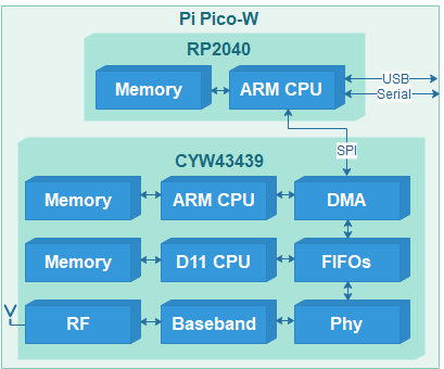
In part 1, I described the low-level hardware & software interface to the Broadcom / Cypress / Infineon CYW43439 WiFi chip, and its close relative, the CYW4343W.

Now we need to initialise the chip, so it is ready to receive network commands and data. This involves sending three files to the chip, and unfortunately there is no simple Application Programming Interface (API) to do this; it is necessary to send a detailed sequence of commands, and if there are any errors, you usually end up with a completely unresponsive WiFi chip.

The first step is to check the Active Low Power (ALP) clock; this involves setting a register, then waiting for the WiFi chip to acknowledge that setting.

bool wifi_init(void)
{
    wifi_reg_write(SD_FUNC_BAK, BAK_CHIP_CLOCK_CSR_REG, SD_ALP_REQ, 1);
    if (!wifi_reg_val_wait(10, SD_FUNC_BAK, BAK_CHIP_CLOCK_CSR_REG, 
                           SD_ALP_AVAIL, SD_ALP_AVAIL, 1))
        return(false);

This wait-and-loop scenario is quite common, so I’ve created a specific function for it:

// Check register value every msec, until correct or timeout
bool wifi_reg_val_wait(int ms, int func, int addr, uint32_t mask, uint32_t val, int nbytes)
{
    bool ok;
    
    while (!(ok=wifi_reg_read_check(func, addr, mask, val, nbytes)) && ms--)
        usdelay(1000);
    return(ok);
}

// Read & check a masked value, return zero if incorrect
bool wifi_reg_read_check(int func, int addr, uint32_t mask, uint32_t val, int nbytes)
{
    return((wifi_reg_read(func, addr, nbytes) & mask) == val);
}

A value is obtained from the register, masked with an AND-function, then compared with the required value. If the comparison is false, the code delays for one millisecond, then tries again, until the given time (in milliseconds) has expired.

This raises the question as to what the code should do when it encounters an error such as this; should it try to re-send the command? In practice, the timeout generally means that the internal state of the chip is incorrect; for example, there may have been a bug in the code, or a power glitch, and the only way to correct this situation is to re-power the chip, and start again – fortunately the initialisation process is quite fast (it only takes a few seconds) so this isn’t a major problem.

Assuming the ALP check passes, there are some more register write cycles that I can’t explain in detail, as I don’t have access to any information about the chip that isn’t publicly available.

We then make 2 writes to registers in banked memory, that do deserve more explanation.

#define BAK_BASE_ADDR           0x18000000
#define SRAM_BASE_ADDR          (BAK_BASE_ADDR+0x4000)
#define SRAM_BANKX_IDX_REG      (SRAM_BASE_ADDR+0x10)
#define SRAM_BANKX_PDA_REG      (SRAM_BASE_ADDR+0x44)

wifi_bak_reg_write(SRAM_BANKX_IDX_REG, 0x03, 4);
wifi_bak_reg_write(SRAM_BANKX_PDA_REG, 0x00, 4);

The backplane function can only access a 32K block in the WiFi RAM, so the two addresses we’re writing (18004010 and 18004044 hex) are outside its access range, and we have to use bank-switching. There is a simple check to see if the bank has changed since the last access, in which case no switching is needed:

#define SB_32BIT_WIN    0x8000
#define SB_ADDR_MASK    0x7fff
#define SB_WIN_MASK     (~SB_ADDR_MASK)

// Set backplane window if address has changed
void wifi_bak_window(uint32_t addr)
{
    static uint32_t lastaddr=0;

    addr &= SB_WIN_MASK;
    if (addr != lastaddr)
        wifi_reg_write(SD_FUNC_BAK, BAK_WIN_ADDR_REG, addr>>8, 3);
    lastaddr = addr;
}

// Write a 1 - 4 byte value via the backplane window
int wifi_bak_reg_write(uint32_t addr, uint32_t val, int nbytes)
{
    wifi_bak_window(addr);
    return(wifi_reg_write(SD_FUNC_BAK, addr, val, nbytes));
}

We can now load the binary ARM firmware into the WiFi processor; it is in a file that is unique to the specific Wifi chip, so different files are needed for the CYW43439 and CYW4343w; these are the only differences in the way the chips are programmed.

const unsigned char fw_firmware_data[] = {
0x00,0x00,0x00,0x00,0x65,0x14,0x00,0x00,0x91,0x13,0x00,0x00,0x91,0x13,0x00,0x00,0x91,0x13,0x00,0x00,0x91,0x13,0x00,0x00,0x91,0x13,0x00,0x00,0x91,0x13,0x00,0x00,0x91,0x13,0x00,0x00,0x91,0x13,0x00,0x00,
..and so on..
}
const unsigned int fw_firmware_len = sizeof(fw_firmware_data);

wifi_data_load(SD_FUNC_BAK, 0, fw_firmware_data, fw_firmware_len);

As previously mentioned, the backplane can only access a 32K block, and each SPI access to the backplane is limited to 64 bytes, so the data loading function walks though the memory in 64-byte blocks, and when 32K is reached, the access window is moved up, and the loading resumes at address 0.

#define MAX_BLOCKLEN    64

// Load data block into WiFi chip (CPU firmware or NVRAM file)
int wifi_data_load(int func, uint32_t dest, const unsigned char *data, int len)
{
    int nbytes=0, n;
    uint32_t oset=0;
    
    wifi_bak_window(dest);
    dest &= SB_ADDR_MASK;
    while (nbytes < len)
    {
        if (oset >= SB_32BIT_WIN)
        {
            wifi_bak_window(dest+nbytes);
            oset -= SB_32BIT_WIN;
        }
        n = MIN(MAX_BLOCKLEN, len-nbytes);
        wifi_data_write(func, dest+oset, (uint8_t *)&data[nbytes], n);
        nbytes += n;
        oset += n;
    }
    return(nbytes);
}

After a delay to allow the WiFi chip to settle, the next item to be loaded is the non-volatile RAM (NVRAM) data. This is in the form of a C character array, with each entry being null-terminated, e.g.

const unsigned char fw_nvram_data[0x300] = {
    "manfid=0x2d0"  "\x00"
    "prodid=0x0727" "\x00"
    "vendid=0x14e4" "\x00"
    ..and so on..
}
const unsigned int fw_nvram_len = sizeof(fw_nvram_data);

Loading this file uses the same function as the firmware, with a different base, and a write-cycle to confirm the file length:

#define NVRAM_BASE_ADDR     0x7FCFC

wifi_data_load(SD_FUNC_BAK, NVRAM_BASE_ADDR, fw_nvram_data, fw_nvram_len);
n = ((~(fw_nvram_len / 4) & 0xffff) << 16) | (fw_nvram_len / 4);
wifi_reg_write(SD_FUNC_BAK, SB_32BIT_WIN | (SB_32BIT_WIN-4), n, 4);

Now it is necessary to reset the WiFi processor core, wait for the indication that the High Throughput (HT) clock is available, then wait for an ‘event’ that signals the device is ready. The most common fault I experienced when developing the code was that it gets stuck at this point, waiting for a confirmation that never comes.

// Reset, and wait for High Throughput (HT) clock ready
wifi_core_reset(false);
if (!wifi_reg_val_wait(50, SD_FUNC_BAK, BAK_CHIP_CLOCK_CSR_REG, 
                              SD_HT_AVAIL, SD_HT_AVAIL, 1))
    return(false);
// Wait for backplane ready
if (!wifi_rx_event_wait(100, SPI_STATUS_F2_RX_READY))
    return(false);

Events are the main way that the WiFi chip sends signals or data asynchronously to the RP2040; for a detailed description of how they work, see the next part.

Once the system has signalled it is ready, the Country Locale Matrix (CLM) file has to be loaded. This binary file limits the WiFi parameters (e.g. transmit power level) to be within the regulatory constraints for the specific RF hardware and locale.

const unsigned char fw_clm_data[] = {
	0x42,0x4C,0x4F,0x42,0x3C,0x00,0x00,0x00,0xFA,0x69,0xE0,0xBB,
	0x01,0x00,0x00,0x00,0x02,0x00,0x00,0x00,0x00,0x00,0x00,0x00,
    ..and so on..
};
const unsigned int fw_clm_len = sizeof(fw_clm_data);

wifi_clm_load(fw_clm_data, fw_clm_len);

The loading function uses a specific structure to send IOCTL data blocks to the WiFi chip, with flags to mark the beginning & end of the sequence:

#define MAX_LOAD_LEN        512

typedef struct {
	uint16_t flag;
	uint16_t type;
	uint32_t len;
	uint32_t crc;
} CLM_LOAD_HDR;

typedef struct {
    char req[8];
    CLM_LOAD_HDR hdr;
} CLM_LOAD_REQ;

// Load CLM
int wifi_clm_load(const unsigned char *data, int len)
{
    int nbytes=0, oset=0, n;
    CLM_LOAD_REQ clr = {.req="clmload", .hdr={.type=2, .crc=0}};
    
    while (nbytes < len)
    {
        n = MIN(MAX_LOAD_LEN, len-nbytes);
        clr.hdr.flag = 1<<12 | (nbytes?0:2) | (nbytes+n>=len?4:0);
        clr.hdr.len = n;
        ioctl_set_data2((void *)&clr, sizeof(clr), 1000, (void *)&data[oset], n);
        nbytes += n;
        oset += n;
    }
    return(nbytes);
}

Example program

To show all this code in action, we can run our first complete program;

// PicoWi blinking LED test

#include <stdint.h>
#include <stdbool.h>
#include <stdio.h>
#include "picowi_pico.h"
#include "picowi_spi.h"
#include "picowi_init.h"

int main() 
{
    uint32_t led_ticks;
    bool ledon=false;
    
    io_init();
    printf("PicoWi LED blink\n");
    set_display_mode(DISP_INFO);
    if (!wifi_setup())
        printf("Error: SPI communication\n");
    else if (!wifi_init())
        printf("Error: can't initialise WiFi\n");
    else
    {
        ustimeout(&led_ticks, 0);
        while (1)
        {
            if (ustimeout(&led_ticks, 500000))
                wifi_set_led(ledon = !ledon);
        }
    }
}

This sets up the WiFi chip as described above, prints the 6-byte MAC address, then just loops, flashing the LED that is attached to the Wifi chip at 1 Hz.

The display_mode function controls how much diagnostic information you might want to see, using a bitfield so you can combine multiple options:

// Display mask values
#define DISP_NOTHING    0       // No display
#define DISP_INFO       0x01    // General information
#define DISP_SPI        0x02    // SPI transfers
#define DISP_REG        0x04    // Register read/write
#define DISP_SDPCM      0x08    // SDPCM transfers
#define DISP_IOCTL      0x10    // IOCTL read/write
#define DISP_EVENT      0x20    // Event reception
#define DISP_DATA       0x40    // Data transfers

This can potentially provide a lot of diagnostic information, the main limitation being the speed of the console display – I use a serial link at 460800 baud, since the default of 9600 is much too slow. To see some of the internal workings of PicoWi, try:

set_display_mode(DISP_INFO|DISP_REG|DISP_IOCTL);

You can call this function multiple times with different mode values, to concentrate the diagnostic information on a specific area of interest, and avoid displaying a lot of unwanted information while the WiFi chip is being initialised.

The other unusual feature is the use of the ustimeout function, which I’ve used it in place of the more conventional delay function call, as I don’t want the delay to block all other CPU activity. In a simple program this isn’t an issue, but in later examples I want to do other things (such as checking for events) while waiting for the LED to blink, so can’t use a simple delay.

The ustimeout function takes two arguments; a pointer to a variable, and a timeout value in microseconds (zero if immediate). When the specified time has elapsed, the function returns a non-zero value and reloads the variable with the current time. So you can add extra function calls to the main loop, without affecting the LED blinking.

The code to control the LED uses a single Device I/O Control (IOCTL) call with 2 arguments; the first is a bit-mask, and the second is the value:

#define SD_LED_GPIO     0

// Set WiFi LED on or off
void wifi_set_led(bool on)
{
    ioctl_set_intx2("gpioout", 10, 1<<SD_LED_GPIO, on ? 1<<SD_LED_GPIO : 0);
}

For details on how to build & run this example program, see the introduction.

IOCTL calls are the primary mechanism for high-level communication with the WiFi chip; see the next part for a detailed description.

Copyright (c) Jeremy P Bentham 2022. Please credit this blog if you use the information or software in it.

The WiFi interface on the Pico W uses the Broadcom/Cypress/Infineon CYW43439; this is a ‘full’ Media Access and Control (MAC) chip, so in theory you can just tell it to join a network, or send a block of data, and it’ll handle all the low-level operations.

However, in practice there is a lot more complication than that, and it takes a very large number of carefully-timed commands before the chip will start up, let alone do anything useful. This is because it actually contains two processors (ARM M3 and D11), each with their own memory and I/O, and they both have to be programmed before any network operations can start.

The CYW43439 is part of a large family of 43xxx wireless interfaces; most use PCI, USB or SDIO interface for communications with a host processor, but in this case communications is via a Serial Peripheral Interface (SPI) that is half-duplex, i.e. a single wire is used to carry commands & data to the WiFi chip, and also the responses from that chip, as described in the device datasheet.

SPI interface

This excerpt from the Pico-W circuit diagram shows the interface between the CYW43439 WiFi chip and the RP2040 CPU. The connections on the WiFi chip are labelled as if there were an SDIO interface, since they are dual-function:

On chips with dual interfaces, the state of DATA2 at power-up determines which interface is to be used; for SPI, this pin must be held low, before REG_ON is set high to power up the chip.

A single data line is shared between CMD for commands & data going to the WiFi chip, and DATA0 for the returned responses. Just in case there is a clash of I/O (e.g. both the CPU and WiFi chip transmitting at the same time) there is a 470 ohm protection resistor in series with DATA0.

The chip-select line is as usual for SPI interfaces; when it is high, the WiFi interface is disconnected from the data lines. This allows the over-worked data line to be used for a third purpose, namely interrupt request (IRQ) to the RP2040 CPU; when the interface is idle, IRQ is normally low, but goes high when the WiFi chip has some data to send (e.g. a new data packet has been received). To ensure that the IRQ line doesn’t interfere with communications, it is connected via a 10K resistor.

Debug with CYW4343W

When developing this software, there was a major problem; the Pico-W components and PCB tracks are so fine that I couldn’t attach an oscilloscope or logic analyser to the SPI connections. This makes debugging the low-level drivers very difficult, especially when programming the PIO peripheral in the RP2040.

The solution I adopted was to add a second CYW43xxx interface to the Pico; unfortunately I couldn’t find a convenient CYW43439 module, but Avnet sell an FPGA add-on board (part number AES-PMOD-MUR-1DX-G) with a Murata 1DX module containing a CYW4343W. This is sufficiently similar to the 43439 that no code modifications are required, just a different firmware file, as described in part 2 of this post.

I’ve had to tweak the resistor values slightly; this is because D0 – D4 pins on the module have 10K pullup resistors, so R2 has to be lower to compensate.

The choice of GPIO pins is completely arbitrary, since the code can work with any pin taking any function; I chose D0 – D3 as GP16 – GP19, since it will allow me to experiment with an SDIO interface at a future date. If you are only interested in emulating the standard Pico-W interface, then the connections to GP16 – GP18 can be omitted, since the SPI select line (D2) has a pull-down resistor.

The resulting circuitry fits very neatly onto a Pico prototyping board; by keeping the connections short, it works fine with SPI speeds up to 16 MHz. The only problems I encountered in constructing the hardware were that the PMOD connector has an unusual pin-numbering, and is mis-labelled as Bluetooth.

Using this setup, it is easy to capture the SPI waveforms; here is an oscilloscope trace using a (relatively leisurely) 2 MHz clock for clarity.

This shows a 4-byte command on the MOSI line, followed by a 4-byte MISO response, which also appears on the MOSI line, due to the 470 ohm resistor linking the two.

SPI software

Normally we’d just use the RP2040 built-in SPI controller to access the WiFi chip, but that has specific sets of pins it can use, which differ from those that are connected to the chip. This isn’t a major problem, as we can use the built-in Programmble I/O (PIO) to do the transfers, but initially I’d just like to check that the hardware works, before diving into PIO programming. So the first step is to write a ‘bit-bashed’ driver, that uses direct access to the I/O bits.

The write-cycle is quite conventional, where a bit (most-significant bit first) is put onto the data line, and the clock is toggled high then low:

// Write data to SPI interface
void spi_write(uint8_t *data, int nbits)
{
    uint8_t b=0;
    int n=0;

    io_mode(SD_CMD_PIN, IO_OUT);
    usdelay(SD_CLK_DELAY);
    b = *data++;
    while (n < nbits)
    {
        IO_WR(SD_CMD_PIN, b & 0x80);
        IO_WR(SD_CLK_PIN, 1);
        b <<= 1;
        if ((++n & 7) == 0)
            b = *data++;
        IO_WR(SD_CLK_PIN, 0);
    }
    usdelay(SD_CLK_DELAY);
    io_mode(SD_CMD_PIN, IO_IN);
    usdelay(SD_CLK_DELAY);
}

If the command is a data-read, the data is read immediately, then the clock is toggled high and low. This is unusual, and can cause confusion in some protocol decoders:

// Read data from SPI interface
void spi_read(uint8_t *data, int nbits)
{
    uint8_t b;
    int n=0;

    data--;
    while (n < nbits)
    {
        b = IO_RD(SD_DIN_PIN);
        IO_WR(SD_CLK_PIN, 1);
        if ((n++ & 7) == 0)
            *++data = 0;        
        *data = (*data << 1) | b;
        IO_WR(SD_CLK_PIN, 0);
    }
 }

A write-cycle to the WiFi chip involves creating a command message as described in the data sheet, setting chip-select (CS) low, and transferring that message, followed by the data.

#define SWAP16_2(x) ((((x)&0xff000000)>>8) | (((x)&0xff0000)<<8) | \
                    (((x)&0xff00)>>8)      | (((x)&0xff)<<8))
#define SD_FUNC_BUS         0
#define SD_FUNC_BAK         1
#define SD_FUNC_RAD         2
#define SD_FUNC_SWAP        4
#define SD_FUNC_BUS_SWAP    (SD_FUNC_BUS | SD_FUNC_SWAP)
#define SD_FUNC_MASK        (SD_FUNC_SWAP - 1)

typedef struct
{
    uint32_t len:11, addr:17, func:2, incr:1, wr:1;
} SPI_MSG_HDR;

// SPI message
typedef union
{
    SPI_MSG_HDR hdr;
    uint32_t vals[2];
    uint8_t bytes[2048];
} SPI_MSG;

// Write a data block using SPI
int wifi_data_write(int func, int addr, uint8_t *dp, int nbytes)
{
    SPI_MSG msg={.hdr = {.wr=1, .incr=1, .func=func&SD_FUNC_MASK,
                         .addr=addr, .len=nbytes}};
    if (func & SD_FUNC_SWAP)
        msg.vals[0] = SWAP16_2(msg.vals[0]);
    io_out(SD_CS_PIN, 0);
    usdelay(SD_CLK_DELAY);
    if (nbytes <= 4)
    {
        memcpy(&msg.bytes[4], dp, nbytes);
        spi_write((uint8_t *)&msg, 64);
    }
    else
    {
        spi_write((uint8_t *)&msg, 32);
        usdelay(SD_CLK_DELAY);
        spi_write(dp, nbytes*8);
    }
    usdelay(SD_CLK_DELAY);
    io_out(SD_CS_PIN, 1);
    usdelay(SD_CLK_DELAY);
    return(nbytes);
}

The command header contains:

• Length: byte-count of data
• Address: location to receive the data
• Function number: destination for the transfer
• Increment: flag to enable address auto-increment
• Write: flag to indicate a write-cycle

The unusual item is the function number, that selects which peripheral within the WiFi chip will receive the data; a value of 0 selects the SPI interface, 1 the backplane, and 2 the radio. Functions 0 & 1 are limited to a maximum size of 64 bytes, and are generally used for device configuration, whilst function 2 is used for transferring network data, which can be up to 2048 bytes. I’ve also created a dummy function 4, which is used to signal that a word-swap is required, when the chip is uninitialised.

The read cycle has a similar structure:

// Read data block using SPI
int wifi_data_read(int func, int addr, uint8_t *dp, int nbytes)
{
    SPI_MSG msg={.hdr = {.wr=0, .incr=1, .func=func&SD_FUNC_MASK,
                         .addr=addr, .len=nbytes}};
    uint8_t data[4];

    if (func & SD_FUNC_SWAP)
        msg.vals[0] = SWAP16_2(msg.vals[0]);
    else if (func == SD_FUNC_BAK)
        msg.hdr.len += 4;
    io_out(SD_CS_PIN, 0);
    usdelay(SD_CLK_DELAY);
    spi_write((uint8_t *)&msg, 32);
    io_mode(SD_CMD_PIN, IO_IN);
    usdelay(SD_CLK_DELAY);
    if (func == SD_FUNC_BAK)
        spi_read(data, 32);
    usdelay(SD_CLK_DELAY);
    spi_read(dp, nbytes*8);
    usdelay(SD_CLK_DELAY);
    io_mode(SD_CMD_PIN, IO_OUT);
    io_out(SD_CS_PIN, 1);
    return(nbytes);
}

When making a ‘backplane’ read, the first 4 return bytes are discarded; they are padding to give the remote peripheral time to respond.

Now that we have the necessary read/write functions, we can perform a simple check to see if the WiFi chip is responding. The data sheet describes several ‘gSPI registers’ and the ‘test read-only’ register at address 0x14 has the defined constant 0xFEEDBEAD. The first attempt to read this register generally fails, but subsequent reads should return the desired value:

#define SPI_TEST_VALUE 0xfeedbead
bool ok=0;
for (int i=0; i<4 && !ok; i++)
{
    usdelay(2000);
    val = wifi_reg_read(SD_FUNC_BUS_SWAP, 0x14, 4);
    ok = (val == SPI_TEST_VALUE);
}
if (!ok)
    printf("Error: SPI test pattern %08lX\n", val);

Next we need to configure the SPI interface to our preferences, using register 0, as described in the datasheet. The main change is to eliminate the awkward byte-swapping, but to do that, we need to send a byte-swapped command:

// Write a register using SPI
int spi_reg_write(int func, uint32_t addr, uint32_t val, int nbytes)
{
    if (func&SD_FUNC_SWAP && nbytes>1)
        val = SWAP16_2(val);
    return(wifi_data_write(func, addr, (uint8_t *)&val, nbytes));
}

wifi_reg_write(SD_FUNC_BUS_SWAP, SPI_BUS_CONTROL_REG, 0x204b3, 4);

Now we can re-read the test register without the awkward byte-swapping:

wifi_reg_read(SD_FUNC_BUS, 0x14, 4);

Another parameter we’ve set is ‘high-speed mode’, which means that reading & writing occur on the rising clock edge.

Using RP2040 PIO

To maximise the speed of SPI transfers, we need to use a peripheral within the RP2040 CPU. Normally this would be an SPI controller, but this can not control the pins that are connected to the WiFi chip, so we have to use the Programmable I/O (PIO) peripheral instead.

There are plenty of online tutorials explaining how PIO works; it is basically a small state-machine that is programmed in assembly-language. It operates in a highly deterministic fashion, at a rate of up to 125M instructions per second, so is ideally suited to handling the SPI interface.

I wanted to use the PIO as a direct replacement for the bit-bashed spi_read and spi_write functions described above, so the PIO program is:

; Pico PIO program for half-duplex SPI transfers
.program picowi_pio
.side_set 1
.wrap_target
.origin 0
public stall:               ; Stall here when transfer complete
    pull            side 0  ; Get byte to transmit from FIFO
loop1:
    nop             side 0  ; Idle with clock low
    in pins, 1      side 0  ; Fetch next Rx bit
    out pins, 1     side 0  ; Set next Tx bit 
    nop             side 1  ; Idle high
    jmp !osre loop1 side 1  ; Loop if data in shift reg
    push            side 0  ; Save Rx byte in FIFO
.wrap
; EOF

The origin statement ensures the program is loaded at address zero, rather than the default, which is to load it at the top of program memory.

The ‘pull’ instruction fetches an 8-bit value from the transmit first-in first-out (FIFO) buffer, then there is a loop to output & input the individual bits of that byte until the transmit shift register is empty, and the receive register is full, so the latter can be pushed onto the receive FIFO.

So for SPI write, the associated C code just needs to keep the 4-entry transmit FIFO topped up with the outgoing data, and discard the incoming data, so the receive FIFO doesn’t overflow.

static PIO my_pio = pio0;
uint my_sm = pio_claim_unused_sm(my_pio, true);
io_rw_8 *my_txfifo = (io_rw_8 *)&my_pio->txf[0];

// Write data block to SPI interface,
// When complete, set data pin as I/P (so it is available for IRQ)
void pio_spi_write(unsigned char *data, int len)
{
    config_output(1);
    pio_sm_clear_fifos(my_pio, my_sm);
    while (len)
    {
        if (!pio_sm_is_tx_fifo_full(my_pio, my_sm))
        {
            *my_txfifo = *data++;
            len --;
        }
        if (!pio_sm_is_rx_fifo_empty(my_pio, my_sm))
            pio_sm_get(my_pio, my_sm);
    }
    while (!pio_sm_is_tx_fifo_empty(my_pio, my_sm) || !pio_complete())
    {
        while (!pio_sm_is_rx_fifo_empty(my_pio, my_sm))
            pio_sm_get(my_pio, my_sm);
    }
    pio_sm_get(my_pio, my_sm);
    config_output(0);
}

The SPI read code fills the transmit FIFO with null bytes, and fetches the incoming data from the receive FIFO:

// Read data block from SPI interface
void pio_spi_read(unsigned char *data, int rxlen)
{
    int txlen=rxlen;
    pio_sm_clear_fifos(my_pio, my_sm);
    while (rxlen > 0 || !pio_complete())
    {
        if (txlen>0 && !pio_sm_is_tx_fifo_full(my_pio, my_sm))
        {
            *my_txfifo = 0;
            txlen--;
        }
        if (!pio_sm_is_rx_fifo_empty(my_pio, my_sm))
        {
            *data++ = pio_sm_get(my_pio, my_sm);
            rxlen--;
        }
    }
}

Since the reading of a WiFi register involves an SPI write cycle closely followed by a read cycle, it is important that the write cycle is complete before the read cycle starts. This issue proved to be the biggest problem with the PIO code; it is easy to detect when the transmit FIFO is empty, but the code must carry on waiting until the last bit of the last byte has been shifted out. This means that I have to use an explicitly-coded loop in the assembly language, with a check of shift-register-empty, rather than using the auto-load capability of the input & output instructions.

The other tricky issue was how the assembly-language program should signal to the C program that the output-shift is complete. In theory, I can use an IRQ flag to do this signalling, but in practice I could not make that work reliably – the technique would only work at specific clock frequencies, which suggested that there might be a critical race between the two sets of code. The problem with timing-sensitive code is that a small unrelated change to the main program (e.g. addition of an interrupt) can cause the code to fail in a manner that is very difficult to diagnose, so it is essential that the code works reliably over a wide range of SPI frequencies.

The solution I adopted is encapsulated in the pio_complete function:

// Check to see if PIO transfer complete (stalled at FIFO pull)
static inline int pio_complete(void)
{
    return(my_pio->sm[my_sm].addr == picowi_pio_offset_stall);
}

This compares the current PIO execution address with the ‘stall’ label in the PIO code; if the transmit FIFO is empty, and this comparison is true, then the PIO is stalled waiting for more data, having shifted out everything it was given.

In a single-threaded program, it won’t be too difficult to keep the transmit FIFO topped up, and the receive FIFO emptied, so there is no risk of an overflow or underflow causing problems. However, this is more difficult when the program is multi-tasking, so it will be necessary to add Direct Memory Access (DMA) transfers to the current code.

Update: increasing SPI speed

The code-update has a much-improved SPI interface driver, which can achieve an SPI speed up to 62 MHz. There were 2 obstacles to achieving this speed; the first was the absence of DMA, which is easily rectified, then there was a more complicated issue due to the way the hardware is designed.

Direct Memory Access

DMA isn’t difficult, since the Pico SDK provides some really helpful functions, e.g. to set up transmission from a PIO channel:

uint wifi_tx_dma_dreq, wifi_tx_dma_dreq;
dma_channel_config cfg;
   
wifi_tx_dma_dreq = pio_get_dreq(wifi_pio, wifi_sm, true);
wifi_tx_dma_chan = dma_claim_unused_channel(true);
cfg = dma_channel_get_default_config(wifi_tx_dma_chan);
channel_config_set_transfer_data_size(&cfg, DMA_SIZE_8);
channel_config_set_read_increment(&cfg, true);
channel_config_set_write_increment(&cfg, false);
channel_config_set_dreq(&cfg, wifi_tx_dma_dreq);
dma_channel_configure(wifi_tx_dma_chan, &cfg, &wifi_pio->txf[wifi_sm], NULL, 8, false);

Then to initiate a DMA transfer:

dma_channel_transfer_from_buffer_now(wifi_tx_dma_chan, dp, nbits / 8);
dma_channel_wait_for_finish_blocking(wifi_tx_dma_chan);

I’ve chosen to stall (‘block’) the CPU until the DMA transfer is complete, but it could carry on executing code while the transfer progresses.

SPI speedup

Pi Pico-W interface to CYW43439

To save on I/O pins, the Pi Pico designer decided to use one pin to carry the incoming data from the CPU, the outgoing data to the CPU, and the interrupt signal. To avoid the possibility of an I/O clash when handling these 3 signals, the incoming & outgoing data pins aren’t directly connected together; there is a 470 ohm resistor in series with the data input.

In the previous code, we could ignore this resistor, since at a low data rate it has no real effect. However, as we increase the speed, the series resistance combines with the parallel (‘shunt’) capacitance to slow down the edges of the received data, resulting in errors. The obvious way to handle this is to slow the clock down, but since most SPI drivers work on the principle of simultaneously sending and receiving each byte, this means that SPI transmission is slowed down as well.

My solution is to split the SPI code into 2 separate functions, so the PIO either transmits or receives, and the slower reception doesn’t hinder the faster transmission.

The resulting PIO transmit code is simplified, so is much faster:

.origin 0
public stall:                   ; Stall here when transfer complete

; Write data to SPI (42 MHz SPI clock, if divisor is set to 1)
public writer:
    pull                side 0  ; Get byte to transmit from FIFO
  wrloop:
    nop                 side 0  ; Delay (if deleted, SPI clock is 63 MHz)
    out pins, 1         side 0  ; Set next Tx bit 
    jmp !osre wrloop    side 1  ; Loop if data in shift reg
.wrap

One of the difficulties with transmission is how to determine when it has completely finished, i.e. with both the FIFO and the shift register empty. For this reason I use an OSRE (output shift register empty) loop, such that I can detect when the transfer is complete using the pio_complete function described above.

As written above, the SPI runs at 41.7 MHz (125 MHz / 3), but it will also work at 62.5 MHz (125 MHz / 2) by deleting one of the ‘nop’ instructions, though this does violate the timing specification of the CYW43439, which is limited to 50 MHz. [Note: I am aware of the ability of the fractional divider to generate a more exact 50 MHz frequency, however this is done by inserting occasional delays into PIO instructions, so although the net data rate is 50 MHz, there are peaks of 62 MHz, so this still violates the timing specification].

The PIO read code is a lot more relaxed:

; Read data from SPI (25 MHz SPI clock, if divisor is set to 1)
public reader:
    pull                side 0  ; Get byte count from host FIFO
    out x, 32           side 0  ; Copy into x register
  byteloop:
    set y, 7            side 0  ; For each bit in byte..
  bitloop:
    nop                 side 1  ; Delay
    nop                 side 1
    nop                 side 1
    in pins, 1          side 0  ; Input SPI data bit
    jmp y--, bitloop    side 0  ; Loop until byte received
    push                side 0  ; Put byte in host FIFO
    jmp x--, byteloop   side 0  ; Loop until all bytes received
    jmp reader          side 0  ; Loop to start next transfer

This is triggered by putting a byte-count (minus 1) in the FIFO, then the code fetches that number of bytes, and DMA is used to transfer them into from the FIFO into memory. The code needs quite a bit of padding to be slow enough, so I haven’t used auto-push.

I originally put the transmit & receive code in separate PIO instances, but ran into problems with the interaction between the two – I couldn’t get them to share control of the I/O pins. So now I just use a single PIO instance, and select which program to execute by forcing a PIO ‘jump’ command before executing the code, e.g. for writing:

// Write data block to SPI interface
void wifi_spi_write(uint8_t *dp, int nbits)
{
    pio_sm_clear_fifos(wifi_pio, wifi_sm);
    pio_sm_exec(wifi_pio, wifi_sm, pio_encode_jmp(picowi_pio_offset_writer));
    pio_sm_set_consecutive_pindirs(wifi_pio, wifi_sm, SD_CMD_PIN, 1, true);
    dma_channel_transfer_from_buffer_now(wifi_tx_dma_chan, dp, nbits / 8);
    dma_channel_wait_for_finish_blocking(wifi_tx_dma_chan);
}

..and for reading

void wifi_spi_read(uint8_t *dp, int nbits)
{
    int rxlen = nbits / 8;
    int reader = picowi_pio_offset_reader;
    pio_sm_exec(wifi_pio, wifi_sm, pio_encode_jmp(reader));
    dma_channel_transfer_to_buffer_now(wifi_rx_dma_chan, dp, nbits / 8);
    pio_sm_put(wifi_pio, wifi_sm, rxlen - 1);
    dma_channel_wait_for_finish_blocking(wifi_rx_dma_chan);
}

In the next part we’ll initialise the WiFi chip.

Copyright (c) Jeremy P Bentham 2022. Please credit this blog if you use the information or software in it.